The role of data journalists in the scientific process has traditionally been overlooked. However, the most recent pandemic showed how journalism shapes scientific responses and public policy. Thousands of journalists rose to the challenge when the public needed information in order to respond to the rapidly spreading COVID-19 pandemic. Journalists acquired COVID-19 data, visualized it and disseminated their work to help the world contain the virus and flatten the curve.
In order to effectively respond to the pandemic, the world needs a coordinated response driven by accurate, complete data. The data must encompass local outbreaks and be released quickly so action can be taken. Journalists, with experience collecting local information and releasing articles in a timely manner, were well suited to help inform the public. However, by visualizing and analyzing COVID data, journalists became participants in the scientific process rather than simple conveyors of results. Their efforts help data scientists, inform decision-makers and shape a new role for data journalism in crisis situations.
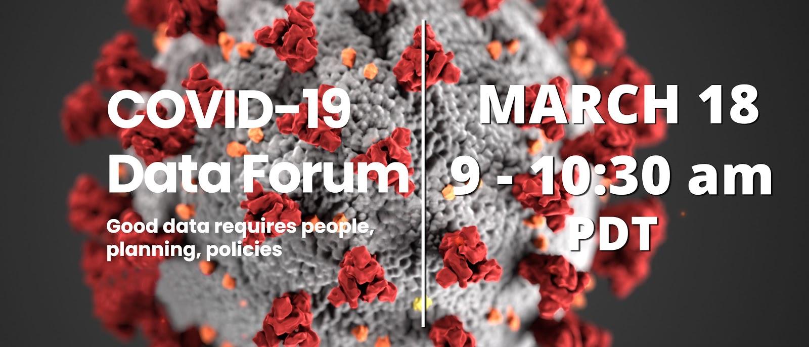
On March 18 the COVID-19 Data Forum, sponsored by the Stanford Data Science Initiative and R Consortium, will host a meeting to discuss how a new breed of data journalists collected quantitative data that helped fight the pandemic. The forum will also discuss how data scientists utilize their resources to create better models.
On November 2 – 7, 2020, the 5th edition of the Brazilian Conference on Data Journalism and Digital Methods (CODA.Br) took place with 50 national and international guest speakers and 16 workshops. CODA.Br is the largest data journalism conference in Latin America and this year was completely virtual.
Open access to all debates, keynotes, lightning talks and presentations of the second edition of the Cláudio Weber Abramo Data Journalism Award is available on the CODA.br website (in Portuguese): https://escoladedados.org/coda2020/
Organized by Open Knowledge Brasil and Escola de Dados (School of Data Brazil), CODA.Br is backed by the support of multiple large scale associations including the Brazilian Association of Investigative Journalism (Abraji), R Consortium, Hivos Institute, Embassy of the Netherlands and the United States Consulate.
With more than 500 attendees, CODA.Br held cutting edge panel discussions covering topics such as avoiding bias in AI with open source tools, Health in journalism and Covid-19, and challenges in the Amazon. Workshops were also held covering a broad range of contemporary subjects like evaluating election data with R and analysis of socioeconomic data in QGIS were held totalling over 24 hours of programming.
Coda.Br made itself even more accessible to the public by offering 150 free passes to build a more diverse, impactful audience. The event attracted participants from 25 states and the federal district in all Brazlian regions. With an average of 73 attendees per workshop, more than half of participants surveyed considered the workshops to be “excellent”.
We can’t wait to see what next year brings for CODA.Br!
On February 7th, 2021, in the very first in the Why R? World Series, Kevin O’Brien of the Why R? Foundation spoke with Nontsikelelo Shongwe, an enthusiastic R user from Eswatini, and co-organizer of the Eswatini UseR meetup group. (Eswatini is located in southeastern Africa, surrounded by South Africa and Mozambique.)
In this interview, Nontsikelelo introduces the landscape of R users in Eswatini and describes her boundary breaking experiences as a young R user. Many thanks to Why R? for giving Nontsikelelo the chance to share her inspiring story.
by Emanuele Guidotti & David Ardia, originally published in the Journal of Open Source Software
In December 2019 the first cases of pneumonia of unknown etiology were reported in Wuhan city, People’s Republic of China.[1] Since the outbreak of the disease, officially called COVID–19 by World Health Organization (WHO), a multitude of papers have appeared. By one estimate, the COVID-19 literature published in January-May 2019 has reached more than 23,000 papers — among the biggest explosions of scientific literature ever.[2]
In response to the COVID-19 pandemic, the White House and a coalition of leading research groups have prepared the COVID-19 Open Research Dataset[3], a resource of over 134,000 scholarly articles about COVID-19, SARS-CoV-2, and related coronaviruses. The Center for Systems Science and Engineering at the Whiting School of Engineering, with technical support from ESRI and the Johns Hopkins University Applied Physics Laboratory, is maintaining an interactive web-based dashboard to track COVID-19 in real time[4]. All data collected and displayed are made freely available through a GitHub repository. [5] A team of over one hundred Oxford University students and staff from every part of the world is collecting information on several different common policy responses governments have taken. The data are aggregated in The Oxford COVID-19 Government Response Tracker[6]. Google and Apple released mobility reports [7][8] to help public health officials. Governments all over the world are releasing COVID-19 data to track the outbreak as it unfolds.
It becomes critical to harmonize the amount of heterogeneous data that have become available to help researchers and policy makers in containing the epidemic. To this end, we developed the COVID-19 Data Hub, designed to aggregate the data from several sources and allow contributors to collaborate on the implementation of additional data providers.[9] The goal of our project is to provide the research community with a unified data hub by collecting worldwide fine-grained case data, merged with exogenous variables helpful for a better understanding of COVID-19.
The data are hourly crunched by a dedicated server and harmonized in CSV format on a cloud storage, in order to be easily accessible from R, Python, MATLAB, Excel, and any other software. The data are available at different levels of granularity: 1) administrative area of top-level, usually countries; 2) states, regions, cantons; 3) cities, municipalities.
The first prototype of the platform was developed in spring 2020, initially as part of a research project that was later published in Springer Nature and showcased on the website of the Joint Research Center of the European Commission. The project was then started at the #CodeVSCovid19 hackathon in March, funded by the Canadian Institute for Data Valorization IVADO in April, won the CovidR contest in May, presented at the European R Users Meeting eRum2020 in June, and published in the Journal of Open Source Software in July. At the time of writing, we count 3.43 million downloads and more than 100 members in the community around the project.
COVID-19 Data Hub has recently received support by the R Consortium[10], the worlwide organization that promotes key organizations and groups developing, maintaining, distributing and using R software as a leading platform for data science and statistical computing.[11]
We are now in the process of establishing close cooperation with professors from the Department of Statistics and Biostatistics of the California State University, in a joint effort to maintain the project.
[3] Wang, Lucy Lu, Kyle Lo, Yoganand Chandrasekhar, Russell Reas, Jiangjiang Yang, Darrin Eide, Kathryn Funk, et al. 2020. “CORD-19: The Covid-19 Open Research Dataset.” arXiv Preprint arXiv:2004.10706.
[4] Dong, Ensheng, Hongru Du, and Lauren Gardner. 2020. “An Interactive Web-Based Dashboard to Track Covid-19 in Real Time.” The Lancet Infectious Diseases 20 (5): 533–34. https://doi.org/10.1016/S1473-3099(20)30120-1.
[6] Hale, Thomas, Samuel Webster, Anna Petherick, Toby Phillips, and Beatriz Kira. 2020. “Oxford Covid-19 Government Response Tracker.” Blavatnik School of Government.
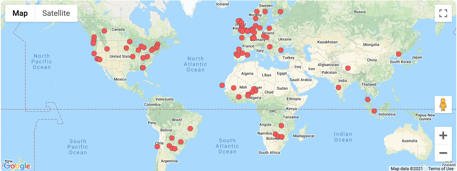
source: R User Groups on meetup.com – 35 countries • 85 groups • 65,200+ members
The R Consortium is excited to announce the 2021 R User Group and Small Conference Support Program (RUGS). We give grants to help R groups around the world organize, share information and support each other. We are now accepting applications!
Because of the limitations of the COVID-19 pandemic on face-to-face meetings, the RUGS program has accordingly shifted its application criteria. The changes are intended to continue to support the energy and creativity of R groups around the globe but focus on virtual and remote solutions.
Changes to the 2021 RUGS program are as follows:
Free access to R Consortium Meetup Pro account
Manage and build events/meetings
Analytics on events and networks
Organize communications with your team
Tiers of grants no longer specified. Draft a proposal including your requested grant amount and purpose
The RUGS 2021 User Group Grants program will award grants in two parts. First, R user groups not affiliated with the RUGS meetup.com Pro will be enrolled with dues covered by the R Consortium for twelve months. Groups will be eligible for a cash award of up to $500.
The RUGS Small Conference Support program will award grants of up to $1,000 to conferences arranged by non-profit or volunteer organizations.
In order to participate in the R Consortium RUGS program (generally smaller organizations), user groups must meet the following criteria:
Use RUGS meetup.com Pro program to announce and track meetings
One blog post per year
Completed W9 Form (US applicants) or Wire Transfer form (non-US)
To participate in the small conference support program (generally slightly larger organizations),conference organizers must agree to the following criteria:
There’s still time! The 2021 RUGS program began accepting applications on January 28, 2021, and will continue to take applications through September 30, 2021.
Citizen science is a critical engine for creating professional tools that become new standards in epidemic outbreak response. The problem is connecting people on the front lines – “COVID-19 response agents” – and people with R language skills.
The R Consortium awarded RECON a grant for $23,300 in the summer of 2019 to develop the RECON COVID-19 challenge, a project aiming to centralise, organise and manage needs for analytics resources in R to support the response to COVID-19 worldwide.
The COVID-19 challenge is an online platform whose goal is to connect members of the R community, R package developers and field agents working on the response to COVID-19 who use R to help them fill-in their R related needs.
Field agents include epidemiologists, statisticians, mathematical modellers and more.
The platform provides a single place for field agents to give feedback in real time on their analytical needs such as requesting specific analysis templates, new functions, new method implementation, etc. These requests are then compiled and organized by order of priority for package developers and members of the R community to browse and help contribute to.
One example is scoringutils. The scoringutils package is currently used by research teams in the UK and US. It is also set to be deployed on a larger scale as part of the evaluation for the US Forecast Hub which is the data source for the official CDC COVID-19 Forecasting page.
As COVID-19 continues to impact people’s lives, we are interested in predicting case trends of the near future. Trying to predict an epidemic is certainly no easy task. While challenging, we explore a variety of modeling approaches and compare their relative performance in predicting case trends. In our methodology, we focus on using data of the past few weeks to predict the data of next week. In this blog, we first talk about the data, how it is formatted and managed, and then describe the various models that we investigated.
Data
The data we use records the number of new cases reported in each county of the U.S everyday. Even though the dataset that we use has much more information, like the number of recovered deaths, etc, the columns that we focus on are “Cases”, “Date”, “State”, and “County”. We combine the “State” and “County” columns together into a single column named “geo.” After that, we decided to use the 2 weeks from 05/21/2020 to 06/03/2020 as training data, to try to predict the median number of cases from 06/04/2020 to 06/10/2020.
We obtain the following table for training set:
To trim down the data, we remove all counties that have less than 10 cases in the 2 training weeks. The final dataset has 1521 counties in total, which is around half of 3,141 total counties in the US.
Projection Method
The first method that we look into is the Friedman’s Supersmoother method. This is a nonparametric estimator based on local linear regression. Using a series of these regressions, the Projection method is able to generate a smoothed line for our time series data. Below is an example of the smoother on COVID case data from King county in Washington State:
As part of our methods for prediction, we use the last 2 points fitted by the smoother to compute a slope, and then use this slope to predict the number of cases for next week. We find that Friedman’s Supersmoother method is consistent and easy to use because it does not require any parameters. However, we have found that outliers can cause the method to sometimes have erratic behavior.
Generalized Linear Model
In this approach, we will use R’s built-in generalized linear model function, glm. GLMs generalize the linear model paradigm by introducing a link function to accommodate data which cannot be fit with a normal distribution. The link function transforms a linear predictor to enable the fit. The type of link function used is specified by the “family” parameter in R’s GLM function. As is usual with count data, we use family=”poisson”. A good introduction can be found at The General Linear Model (GLM): A gentle introduction. One drawback of this approach is that our model could be too sensitive to outliers. To combat against this, we experiment two approaches: Cook’s Distance and Forward Search.
Cook’s Distance:
This method is quite straightforward and can be summarized in 3 steps:
Fit a GLM model.
Calculate Cook’s distance, which measures the influence of each data point, for all 14 points. Remove high influence points where data is far away from the fitted line.
Fit a GLM model again based on the remaining data.
One caveat of this method is that the model might not converge in the first step. Though, such cases are rare if we only use 2 weeks of training data. A longer training period may cause the linear predictor structure to prove too limited and require other methods.
Forward Search:
The Forward Search method is adapted from the second chapter of the text “Robust Diagnostic Regression Analysis,” written by Anthony Atkinson and Marco Riani. In Forward Search, we start with a model fit to a subset of the data. The goal is to start with a model that is very unlikely to be built on data that includes outliers. In our case, there are few enough points that we can build a set of models based on every pair of points; or select a random sample to speed up the process. Out of these, we choose the model that best fits the data. Then, the method will iteratively and greedily select data points to add into the model. In each step, the deviance of the data points from the fitted line is recorded. A steep jump in deviance implies that the newly added data is an outlier. Let’s look at this method in further detail:
1. Find initial model using the following steps:
a. Build models on any combination of 2 data points. Since we have 14 data points in total, we will have (14 choose 2) = 91 candidate models.
b. Compute the trimmed sum squared error of the 14 data points based on each fitted model. (Trimmed here means that we only use the 11 data points with least squared error. The intention is to ignore outliers when fitting)
c. The model with least trimmed squared error is selected as the initial model.
For explanation, let’s assume that this red line below was chosen as the initial model. This means that out of all the pairings of two points, this model, more or less, fit the data the best.
2. Next, we walk through and add the data points to our initial model. The process is as follows:
a. Record the deviance of all 14 data points to the existing model
b. Using the points with the lowest deviations from the current model, select the subset with one additional point for fitting the next model in the sequence
c. Using the newly fit model, repeat this process iteratively on the rest of the data
3. We want to evaluate the results of step 2 by looking at the recorded deviance from each substep. Once there seems to be a steep jump in the recorded deviance (above 1.5 SDs), this indicates that we’ve reached an outlier. The steep jump indicates this because, compared to the model before that does not include the outlier, the newly created model with the outlier shifted the model & the recorded deviance significantly—suggesting that this data point is unlike the rest of the data. Additionally, we can presume that the remaining points after the steep jump are more aligned to the skewed data and could also be treated as outliers.
4. Ignoring the outliers identified in step 3, use the remaining data set as training data for the GLM and fit the final model.
Using this method, we will always be able to get a converged model. However, the first step of selecting the best initial model can be very time consuming and the time complexity is O(N^2), where N is the number of data points in the training set. One way to reduce the runtime is to use a sample of possible combinations. In our example, we may try 10 combinations out of the potential 91 combinations.
Moving Average
Our next approach is a simplified version of Moving Average. For this, we first compute the average of the first training week, and then compute the average of the second training week. Here, we assume that the change in number of cases reported each day has a linear relationship. While simple, using a moving average can obtain decent results with strong performance. Below is a visual representation of this method. The first red point represents the average of the first week and the second represents the average of the second week. The slope of the two points is then used to project the following week.
Results
To evaluate these approaches, we used each method to project the median number of cases for the next week based on the case data from the previous two weeks. In addition, we also analyzed the model in terms of a classification problem—taking a look at whether each model was able to correctly identify whether the case trend was increasing or decreasing. Doing this over all of the counties in our dataset, each method now has a list of 1521 projected medians. Comparing the projections to actual data, we can calculate the observed median error for each county across the methods. The table below displays the percentiles of each method’s list of errors.
Note that it is quite common for the Moving Average and Projection methods to predict a negative number of cases. In those situations, we will force them to predict 0. It is common for both GLM models to produce an extremely large number of cases.
Overall, the GLM model, utilizing Cook’s Distance to find outliers, seems to perform best. This method rarely makes negative predictions and predicts reasonably in most cases. The Moving Average method produced the lowest 100th Percentile, or in other terms, achieved the lowest maximum error. The traditional model-based Cooks Distance method improves on the simple Moving Average approach in most cases. All methods, however, suffer from a number of very unrealistic estimates in some cases. Although the Forward Search method is interesting for its innovative approach, in practice it underperforms and is more costly in terms of compute time.
Now, let’s take a look at the results of our classification problem:
Interestingly, the GLM models seemed to not perform as well when looking at the problem in terms of correctly classifying increasing or decreasing trends universally across the counties. There are two metrics in the table above. The “ROC AUC (>5)” calculates the metric when applied to counties with their previous week’s median case count above 5, whereas the “ROC AUC (>25)” refers to above 25 cases (ROC AUC, which you can read more about here, is a metric for measuring the success of a binary classification model; values closer to 1 indicate better performance). What you can infer from this is that the more simple Moving Average and Projection methods can do better than the GLMs as a blanket approach. However, when looking at counties with more cases, and likely more significant trends, the GLMs prove better. This supports the finding that GLMs can often have erroneous results on insufficient datasets, but good results on datasets with enough quality data. Additionally, we can say that this is a good example to demonstrate that one-size does not fit all when it comes to modelling. Each method has its benefits and it is important to explore those pros and cons when making a decision on what model to use, and when to use it.
Visual Analysis
For a more visual look at the results, we can examine some specific cases. Here, we plot results of the methods on three different scenarios: where the number of cases is less than 50, between 50 and 150, and greater than 150.
In general, it can be seen that the more cases there are in the training set, the more accurate and reasonable are the GLM methods. These perform particularly well when there is a clear trend of increasing or decreasing data. However, the GLM does a poor job when the cases are reported on an inconsistent basis (data on some days, but 0’s on others). In such cases, the fitted curve is “dragged” by the few days of reported data. An example of this is illustrated by the Texas Pecos data in the second figure above.
The Projection method seems to be too subjective to the case counts on the last few days. When there is a sharp decrease on those days, the supersmoother may make negative predictions.
The Moving Average method can be interpreted as a simplified version of the supersmoother. The main difference is that it weights the data of the first and second week equally when making predictions. Therefore, it actually does a slightly better job than the supersmoother.
Effect of Training Period:
To further evaluate these approaches, we can extend the length of the training weeks to see how that might affect the performance of each model. The metric used here is similar to the table from the “Results” section: the median error of the model prediction from the observed data. The results across different training lengths are below:
It is interesting to see that the performance of the GLM-CD model first increases as the length of training data increases (deviances decrease), but later the performance deteriorates once the length of training data is too large.
The following examples illustrate why the performance may deteriorate when the length of training data is too long:
We can see that the GLM model assumes that the trend must be monotone. Once it assumes that the number of cases are increasing, it fails to detect the decreasing number of cases after the outbreak. Therefore, the GLM model is particularly useful when making predictions based solely on the most recent trend. On the contrary, the Projection method is much better at automatically emphasizing the most recent trend, without having to worry about whether the data is monotonic or not, and increasing the length of training data increases its performance in general.
The GLM approach could also be improved by taking into account the presence of a maximum and only using the monotonic portion of the data. For example, the gamlss package and function have a feature that can detect a changepoint and fit a piecewise linear function appropriately. (See Flexible Regression and Smoothing using GAMLSS in R pp 250-253). This would enable us to use a longer time frame when possible in an automated way.
Overall, if we want to use the most recent data for nearcasting based on a GLM model, a 6 week training set seems to be the optimal length. If we were to use a longer period of training data, we might prefer using the Projection method.
Conclusion:
While each model has its advantages and disadvantages, using these approaches can help establish reasonable predictions about future trends in COVID data. Not only can these methods be applied in this specific case, but they can also be used for a number of different use cases involving time series data.
The methodologies used in this analysis were created in R and Spotfire. To run these yourself, simply utilize Spotfire’s data function, which allows you to run R (or python) scripts within the application. For more information on data functions, check out our community, and if you are interested in learning more about our COVID work and what happens under the hood in Spotfire, read here.
Acknowledgments:
A special thanks to Zongyuan Chen, David Katz, and the rest of the team for their contributions.
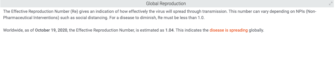
R0, the basic reproduction number, and Rt, the time-varying reproduction number, are quantities used when trying to understand the reproduction rate of the virus. However, both of them are quite difficult to estimate. One glaring issue is the largely unknown prevalence of asymptomatic and presymptomatic cases, which directly impacts our estimates. Another issue is the extent of local versus imported cases (read here for more information on R0/Rt).
A complementary approach to estimating R0 is to consider the reported cases as a random variable, and seek to characterize it directly. This is often done with some form of moving average. Moving average has its advantages—it is familiar and easy to understand. However, it has several disadvantages:
We must choose a bandwidth – the number of days to include in the average. How should we do this?
We do not get an estimate of the stability of the predictions we obtain.
Averages are quite sensitive to outliers, resulting in swings that are difficult to interpret.
At TIBCO, we have been using Friedman’s SuperSmoother (as implemented in R as supsmu) to estimate the epidemic curve of counties, states/provinces, and countries across the world. This has the default option to choose the bandwidth automatically. In most cases, this method appears to match or outperform the moving average method.
One important output that we’d like to get from this exercise is an estimate of the current trend, but this proves challenging for many methods. We have performed a number of experiments to compare various bandwidths and methods for extrapolating into the near future, including the SuperSmoother and GAM/Poisson models (we delve into those results in a separate study). Today, we focus on what we have found to be the most effective method for estimating the current trend: GAMLSS.
GAMLSS
In this blog, we describe our experience with a method called GAMLSS, Generalized Additive Models for Location, Scale and Shape, available in R as package gamlss. Our intention is to provide insight into the overall history, variation, and current trend in COVID data; prediction is not necessarily our focus. This method is described by Stasinopoulos et. al. as a distributional approach—that is, we make an informed guess as to the appropriate distribution to use, and then fit a linear or smooth model via a link function to the data. We use penalized b-splines to fit the time series of new cases with a smooth curve (this method creates a smooth curve adapted to the data). The gamlss package additionally provides easy to use diagnostics to help validate our hypothesis and the fit.
To begin, we apply this method to the daily counts of New Cases from Johns Hopkins as well as the websites of various countries. Initially we use the data by State and Province from around the world. For each geography, defined as ‘country’+’State/Province’, we use the gamlss::fitDist function to find the distribution that best fits the data. We found that “SHAHSo” was a promising choice–“sinh-arcsinh original”. This is a flexible distribution with 4 parameters that control its location, scale and shape.
We fit the data as follows:
Model <- gamlss(New.Cases ~ pb(as.numeric(Date)),
sigma.formula= ~ pb(as.numeric(Date)),
data = train.data,
family=SHASHo())
GAMLSS allows a separate model formula for each of its parameters. On line 1, we model the mu parameter as a smooth curve pb(), which uses a penalized b-spline, with the degree of smoothing selected by cross-validation. The sigma parameter on line 2 is modelled with the same formula. This is a particular advantage of this method, since we do not have to assume constant values for the parameters. Here we have specified a model of the variance changing over time. We see this clearly in the plots below.
Two more parameters, nu and tau, are omitted from this specification, which results in the default, a constant for each of these.
We check the fit by inspecting plot(Model):
These plots show the quantile residuals in various ways. Normalized quantile residuals are transformations of the observed residuals that use the quantiles for the chosen distribution. The effect is that the transformed residuals are normally distributed if the model is correct. You see that this is true when looking at the normal-shaped bell curve in the Density Estimate above, and in the Normal Q-Q plot, where a roughly straight line indicates that the residuals are normally distributed. We find that in many cases, we are able to create adequate models with healthy diagnostics. These models are then used to predict the distribution of values we can expect to see on each date.
Because we have such a model, we use the centiles of the distribution to plot contour lines for any centile. This gives us not only the center of the distribution, but also graphically shows the distribution of confidence intervals. Here is one example:
In this plot, the dots represent the observed values of new cases across the state of Virginia. The output of the GAMLSS model provides a range of outcomes at a certain point in time. Each line in the visualization represents the plot of the nth percentile and the value here is that these can be used to create confidence intervals about the actual trend of the data.
We see an interesting increase in the modelled variance, followed by a relative decrease. We speculate that these high daily counts may indicate highly localized outbreaks in an area, building or event, or timing issues caused by new sets of tests being administered. With sufficient data, the model captures these events as part of its error distribution.
As a means of validating our approach, we use 153 geographic areas for which we developed adequate models. We use 7 days of available data as a hold-out sample, and project our results forward for comparison with the percentiles we predicted. We tag each new observation into the band that it falls into and compare the percentiles of this test data set with the expected percentiles:
Each point (dot) represents a group of observations whose predictions fall into a range of counts. The y-axis is the actual result expressed as a percentile. The line is y=x, perfect agreement between expected and actual.
The observed percentiles agree well with a random set of draws from the predicted distribution. For example, 44% of the actual counts fall below the median predicted for its day and geo. We conclude that extrapolating from such models gives a reasonable expectation of the range of results we are likely to see in the coming week.
We decide to use these percentile plots in TIBCO’s COVID Live Report whenever we are able to fit a good model. In most cases, failures are due to insufficient data, which could be seen as a drawback for the approach. We recognize that the GAMLSS, despite its clear advantages, is not adept at dealing with all types of data. Like any method, it is important to understand its advantages and disadvantages, and when to know how to utilize it.
GAMLSS in TIBCO’s COVID-19 Live Report
Using GAMLSS to fit epidemic curves and predict future cases/deaths over the next week is a new feature in TIBCO’s COVID-19 Live Report. Because GAMLSS does really well at capturing the current trend, a side effect is that the method is able to produce promising estimates about future data. By clicking the “View Forecasts” button on the Live Report’s home page, you are directed to a tab where you can explore the results of our GAMLSS method. On this page, you can choose one or more states/provinces, counties, or countries, and a GAMLSS model will fit to the selected data and provide predictions for the next 7 days. The following is the GAMLSS plot on California’s case counts:
The GAMLSS plot has three lines, one for the 10th, 50th, and 90th centiles. This is a benefit of the GAMLSS method as you are not only able to view the center of distribution, represented by the solid line, but you can also see the distribution of confidence values with the 10th and 90th centiles, represented by the dotted lines. Instead of being limited to just one prediction forecast, the GAMLSS model gives you a range of possibilities of what might happen over the next 7 days, as seen in red.
Conclusion
After some experimentation, we found that the GAMLSS method is an effective approach for understanding trends in COVID data. Due to the method’s unique distributional approach and solid statistical foundations, the GAMLSS improves on other more popular methods like Moving Average for fitting epidemic curves and making predictions. GAMLSS provides a credible estimate of the variance at each point in time and the distribution of expected values in the near future, something lacking in other methods. For more information on GAMLSS, be sure to check out the references below and explore the method on TIBCO’s dashboard.
TIBCO Spotfire is a unique platform that combines advanced visualization and data science techniques. The culmination of its capabilities can be demonstrated in TIBCO’s COVID-19 Visual Analysis Hub. Allowing complex algorithms to run in the background, the application boasts a simple, interactive interface that lets any type of user learn more about the current state of the pandemic. In this blog, we will take a deeper look at the inner workings of the dashboard and explore some of Spotfire’s special functionality, as well as some technical and statistical innovations.
This high-level blog is split into three sections: Data Science Functions, Data Visualization Methods, and Data Engineering(coming soon). Within each section, there will be subsections where you can learn more about specific tools & methods that we used. In addition, some of these subsections will contain links to more detailed blogs—allowing you to read content tailored to your interests.
Feel free to have a look at our Visual Analysis Hub to get a better idea of the work that went behind building it.
Details on Hub’s Data Science Functions
There is much uncertainty about the current state of the pandemic. Recent outbreaks across the world prove that it is hard to pinpoint and contain the coronavirus. Here at TIBCO, our recent work has been focused on trying to make tangible estimates about the actual trends in the data, while also facing the reality that there is only so much that we can be certain about.
One road towards understanding the coronavirus is trying to fit the epidemic curve of the data.
Due to its nature, the case and death data that we observe can be sporadic, confusing, and can take on many different shapes. For creating fit lines, we have adopted two different methodologies: Friedman’s Supersmoother and GAMLSS, a modified version of generalized linear models. This work is done to create the lines seen above, which you can interpret as a summarization of how the data has evolved over time.
Friedman’s Supersmoother:
A large, persistent issue that we continue to face with case growth analysis is the flood of bad/missing data as well as misreported or non-reported data. Some regions have had weird spikes, some have had thousands of cases reported the day after 0 cases were reported (misreporting), etc. In order to overcome these mishaps, we need to use methods that focus on the overall trend of the data and do their best to ignore the noise. As such, we have experimented with different smoothing methods including moving averages and LOESS, but eventually settled on Friedman’s Supersmoother due to its ability to overcome outliers and its lack of hyperparameter tuning. Our implementation of the method used the ‘supsmu’ function found in R’s stats package. Below is a snippet of our code:
Snippet of R Code for Supersmoothing in the COVID-19 Application
In more technical detail, the Supsmu function is a running line smoother that chooses a variable k such that there are k/2 data points on each side of the predicted point. k can be any number between (0.01)*n and n, where n is the number of total data points. If the span itself is specified, the function implements a single smoother with (inputted span)*n used as the span (Friedman, 1984). We run this method for each set of dates in each region using data.table in R and then append the results back into the original data with each region’s corresponding smooth values.
Friedman’s Supersmoother helps to give a relatively noise-free smooth curve that can model the case growth well across regions and differently shaped data. Additionally, we have noticed that the method has adapted well over time. Since surpassing ~six months of data, the input size that is fed into the supersmoother has become quite sufficient and therefore has created increasingly accurate fit curves.
GAMLSS/Nearcasting:
The other method we have explored is GAMLSS, Generalized Additive Models for Location Scale and Shape. This method is valuable and has become one of our favorites because it includes a notion of uncertainty when fitting models on data. Rather than making concrete estimates/predictions about the data, the GAMLSS method provides a range of possible outcomes at any given point in time. You are not just looking at one line that assumes the true shape of the data, but instead you can look and explore multiple estimates of what the trends might look like. For more detailed information about GAMLSS and our processes, we have written a whole blog on the subject, so please check it out!
Another important question that many people want to understand is how COVID-19 trends are going to look like in the near future. To try and answer that question, we experimented with some common and uncommon methods for predicting the amount of coronavirus cases in the next week. An interesting challenge that emerged was the process of choosing an approach for dealing with inconsistent reporting and outliers when modeling. We discovered that some lesser known modeling techniques can prove to be advantageous under certain conditions. You can read the results of our analysis here.
GAMLSS Model Evaluated on California (10/28)
In our Live Report, we use GAMLSS through data functions in Spotfire as a way to fit epidemic curves and make predictions over the next week based on the current trends. Above is an example of running GAMLSS on parts of the San Francisco Bay Area. By choosing counties in the left panel, the coronavirus case data associated with these regions is sent as an input into a data function that creates and runs the models. Inside that data function, we are simply running code written in R that will output three epidemic curves fit to the input data (one for the 10th, 50th, and 90th percentile of the GAMLSS model–the ‘range’ of outcomes). These output lines are then overlaid with the case data on the bottom right panel of our page. Easily configured with visualizations, the data function is capable of running its complex scripts over an interactive user interface. This page can be accessed from the home page by clicking on the “View Forecasts” button. To learn more about how you can integrate R and Python functions with Spotfire, check out our community.
The integration of data science functions in TIBCO’s COVID application demonstrates Spotfire’s ability to coincide statistical analysis with a visual framework. Next, we will take a look at the data visualization techniques used in our dashboard.
Details on Hub’s Visual Functions
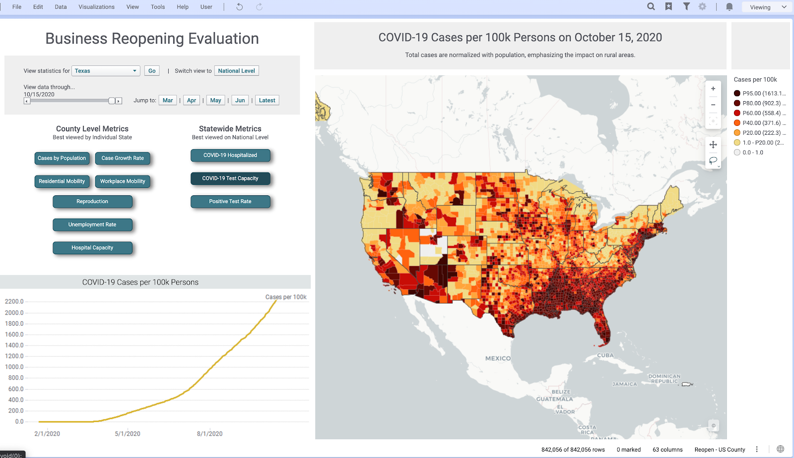
Business Reopenings:
Keeping in mind that each country, and each province within each country, might have different rules and regulations regarding reopening, businesses need a view of all essential metrics that can help them understand the current situation in their region—subsequently assisting them to plan a reopening according to local rules and regulations. To help supplement this decision-making, we created a ‘Business Reopening’ page on our application that provides a one-stop look at all the essential metrics. Through interactive buttons, sliders, and maps, users can evaluate how the pandemic is progressing in their region.
Above is a look at our ‘Business Reopening’ page. This page includes deep drills into unemployment rates, case growth, and mobility—all from different verified sources. In its many interactive features, there is the capability to switch abstraction levels from a geographical perspective, filter results by circling areas on the map, and adjust a slider to look at the analysis at different points in time. Under the hood, when these interactive elements are invoked, the command is sent to a Spotfire data function, which recomputes the analysis and sends the results back to the now updated visualizations.
Here are some examples of different county level metrics we have in the page. All of these can be drilled down into a specific state or at the national level and have detailed views for both:
Reproduction estimates at the County Level
Workplace Mobility in different counties in the State of Virginia
Natural-Language Generation (NLG):
To make the COVID-19 Hub more accessible and understandable for any type of user, we utilize Arria’s NLG (natural-language generation) tools across our application. NLG augments the analysis by building a narrative that is not just charts and graphs, but instead generates detailed insight into what is happening through language.
By gathering information from the data, the NLG tool is able to produce sentences that summarize the data, and do so without making the text sound like it came from a robot. In an excerpt from TIBCO’s website, Arria NLG is described, “Through algorithms and modeling, Arria software replicates the human process of expertly analyzing and communicating data insights—dynamically turning data into written or spoken narrative—at machine speed and massive scale.” The NLG tool is available as a visualization type within Spotfire.
Newspaper style:
The COVID-19 Application uses what is called a Newspaper style layout for visualization within Spotfire. This layout helps in overcoming limitations that can come from a fixed length layout. For example, if a page of an application is non-scrollable, it doesn’t allow you to add as many charts and visualizations as you might want. Instead, you are limited to charts that would be visible to the naked eye and that could fit into the size of a page. The Newspaper style format in Spotfire benefits in making it possible to add as many visualizations as you want and present a logical flow of information that can enrich your insights.
You can easily configure Spotfire’s Page Layout options to extend the page length to make your dashboard newspaper style and take advantage of all the real estate that you can get. This is done by right-clicking on the page navigation bar and configuring the Page Layout to your desire (video tutorial). Here is a quick GIF of how we use newspaper style formats in the COVID-19 Application:
Summary and Future Work
There are many dimensions needed to understand an issue as complex as the coronavirus pandemic. From analyzing hospitalization data to visualizing epidemic curves, TIBCO’s Visual Analysis Hub converges data science, data visualization, and data engineering in one central application. Utilizing Spotfire, these disciplines are used in harmony to deliver insights about the state of the pandemic to just about any type of user. We hope that you were able to learn a bit more about the statistical and technical work that went into our Visual Analysis Hub.
This blog will serve as the central location for any more blogs/updates regarding the development of our COVID dashboard, so be sure to come back and read more about the work that we have done!
Here, again, are the links to the topic-focused blogs:
Thank you to everyone who has contributed to the COVID Visual Analytics Hub and, in particular, a shout out to David Katz, Prem Shah, Neil Kanungo, Zongyuan Chen, Michael O’Connell, and Steven Hillion for their contributions towards creating these blogs and analyses.
The R Consortium’s COVID-19 Working Group is providing a new home for the COVID-19 Data Hub Project. The goal of the COVID-19 Data Hub is to provide the worldwide research community with a unified dataset by collecting worldwide fine-grained case data, merged with external variables helpful for a better understanding of COVID-19.
An initial award of $5,000 will be used to pay storage and maintenance fees for the growing number of international COVID-19 case level data sets. Additionally, the R Consortium will be assuming responsibility for organizing R Community efforts to maintain and develop the site.
When asked about the importance of the project, R Consortium Director Joseph Rickert replied, “I am very pleased that the R Consortium is in a position to make a practical contribution to combating the pandemic. Although, we all hope that the new vaccines will bring the world to some semblance of normality next year, it is likely that the virus will be with us for some time and the need to collect and curate data will continue.”
Created last April by Emanuele Guidotti, doctoral assistant at the Institute for Financial Analysis at the University of Neuchatel, in collaboration with David Ardia, professor at HEC Montreal, the COVID-19 Data Hub Platform is a critical tool for accessing data related to the virus, and looks to establish cooperation and participation with the scientific community around the world. Professors Eric Suess and Ayona Chatterjee of the Department of Statistics and Biostatistics at the California State University East Bay will be joining this effort.
To date, the data has been downloaded 3 million times.
From the full article:
“Working for a research project on COVID-19, I realized the difficulty of accessing data related to the virus,” said Guidotti. The source is heterogeneous: depending on the country, information is disclosed in different languages and formats. To unify them, Guidotti developed the very first prototype of the COVID-19 Data Hub platform in the spring. “This work was originally part of a research paper that was subsequently published in Springer Natureand featured on the Joint Research Center website,” he said. Thanks to the collaboration of David Ardia, the platform received financial support from the Canadian Institute for the Valorization of Data IVADO and HEC Montréal.