

Originally posted on the R Hub blog
This post was contributed by Peter Li. Thank you, Peter!
packageRank is an R package that helps put package download counts into context. It does so via two functions. The first, cranDownloads(), extends cranlogs::cran_downloads() by adding a plot() method and a more user-friendly interface. The second, packageRank(), uses rank percentiles, a nonparametric statistic that tells you the percentage of packages with fewer downloads, to help you see how your package is doing compared to all other CRAN packages.
In this post, I’ll do two things. First, I’ll give an overview of the package’s core features and functions – a more detailed description of the package can be found in the README in the project’s GitHub repository. Second, I’ll discuss a systematic positive bias that inflates download counts.
Two notes. First, in this post I’ll be referring to active and inactive packages. The former are packages that are still being developed and appear in the CRAN repository. The latter are “retired” packages that are stored in the CRAN Archive along with past versions of active packages. Second, if you want to follow along (i.e., copy and paste code), you’ll need to install packageRank (ver. 0.3.5) from CRAN or GitHub:
# CRAN
install.packages("packageRank")

# GitHub
remotes::install_github("lindbrook/packageRank")
library(packageRank)
library(ggplot2)
cranDownloads()
cranDownloads() uses all the same arguments as cranlogs::cran_downloads():
cranlogs::cran_downloads(packages = "HistData")
        date count  package
1 2020-05-01   338 HistData
cranDownloads(packages = "HistData")
        date count  package
1 2020-05-01   338 HistData
The only difference is that `cranDownloads()` adds four features:
Check package names
cranDownloads(packages = "GGplot2")
## Error in cranDownloads(packages = "GGplot2") :
##   GGplot2: misspelled or not on CRAN.
cranDownloads(packages = "ggplot2")
        date count package
1 2020-05-01 56357 ggplot2
This also works for inactive packages in the [Archive](https://cran.r-project.org/src/contrib/Archive):
cranDownloads(packages = "vr")
## Error in cranDownloads(packages = "vr") :
##  vr: misspelled or not on CRAN/Archive.
cranDownloads(packages = "VR")
        date count package
1 2020-05-01    11      VR
Two additional date formats
With cranlogs::cran_downloads(), you can specify a time frame using the from and to arguments. The downside of this is that you must use the “yyyy-mm-dd” format. For convenience’s sake, cranDownloads() also allows you to use “yyyy-mm” or “yyyy” (yyyy also works).
“yyyy-mm”
Let’s say you want the download counts for HistData for February 2020. With cranlogs::cran_downloads(), you’d have to type out the whole date and remember that 2020 was a leap year:
cranlogs::cran_downloads(packages = "HistData", from = "2020-02-01",
  to = "2020-02-29")
With cranDownloads(), you can just specify the year and month:
cranDownloads(packages = "HistData", from = "2020-02", to = "2020-02")
“yyyy”
Let’s say you want the year-to-date counts for rstan. With cranlogs::cran_downloads(), you’d type something like:
cranlogs::cran_downloads(packages = "rstan", from = "2020-01-01",
  to = Sys.Date() - 1)
With cranDownloads(), you can just type:
cranDownloads(packages = "rstan", from = "2020")
Check dates
cranDownloads() tries to validate dates:
cranDownloads(packages = "HistData", from = "2019-01-15",
  to = "2019-01-35")
## Error in resolveDate(to, type = "to") : Not a valid date.
Visualization
cranDownloads() makes visualization easy. Just use plot():
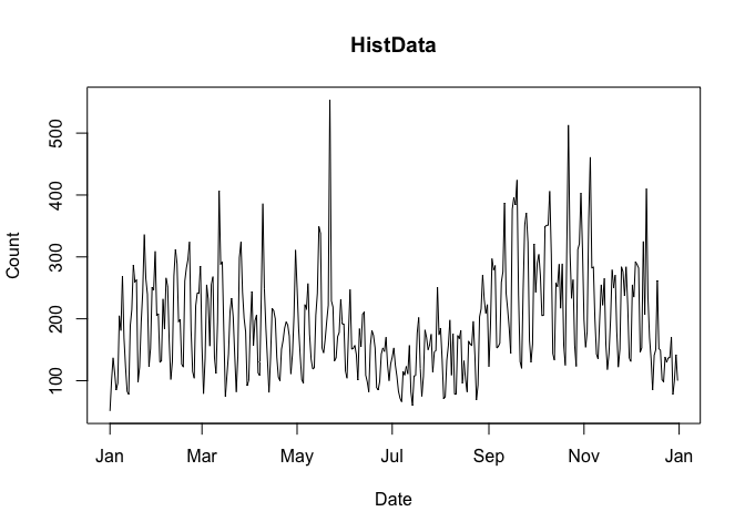
plot(cranDownloads(packages = "HistData", from = "2019", to = "2019"))
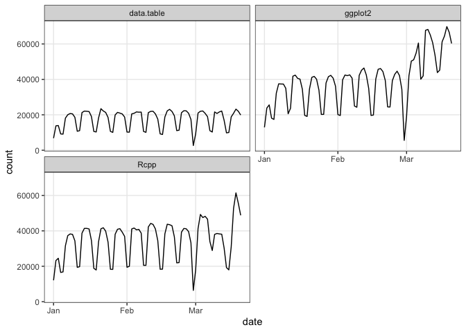
If you pass a vector of package names, plot() will use ggplot2 facets:
plot(cranDownloads(packages = c("ggplot2", "data.table", "Rcpp"),
  from = "2020", to = "2020-03-20"))
If you want to plot those data in a single frame, use `multi.plot = TRUE`:
plot(cranDownloads(packages = c("ggplot2", "data.table", "Rcpp"),
  from = "2020", to = "2020-03-20"), multi.plot = TRUE)
For more plotting options, see the README on GitHub and the plot.cranDownloads() documentation.
packageRank()
packageRank began as a collection of functions I wrote to gauge interest in my cholera package. After looking at the data for this and other packages, the “compared to what?” question quickly came to mind.
Consider the data for the first week of March 2020:
plot(cranDownloads(packages = "cholera", from = "2020-03-01",
  to = "2020-03-07"))
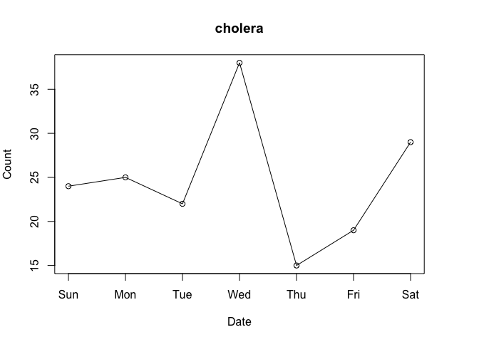
Do Wednesday and Saturday reflect surges of interest in the package or surges of traffic to CRAN? To put it differently, how can we know if a given download count is typical or unusual?
One way to answer these questions is to locate your package in the frequency distribution of download counts. Below are the distributions for Wednesday and Saturday with the location of cholera highlighted:
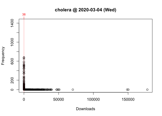
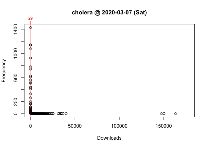
As you can see, the frequency distribution of package downloads typically has a heavily skewed, exponential shape. On the Wednesday, the most “popular” package had 177,745 downloads while the least “popular” package(s) had just one. This is why the left side of the distribution, where packages with fewer downloads are located, looks like a vertical line.
To see what’s going on, I take the log of download counts (x-axis) and redraw the graph. In these plots, the location of a vertical segment along the x-axis represents a download count and the height of a vertical segment represents the frequency of a download count:
plot(packageDistribution(package = "cholera", date = "2020-03-04"))
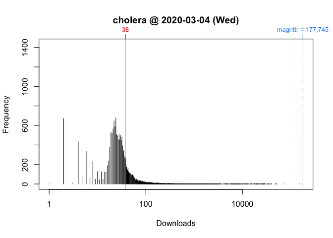
plot(packageDistribution(package = "cholera", date = "2020-03-07"), memoization = FALSE)
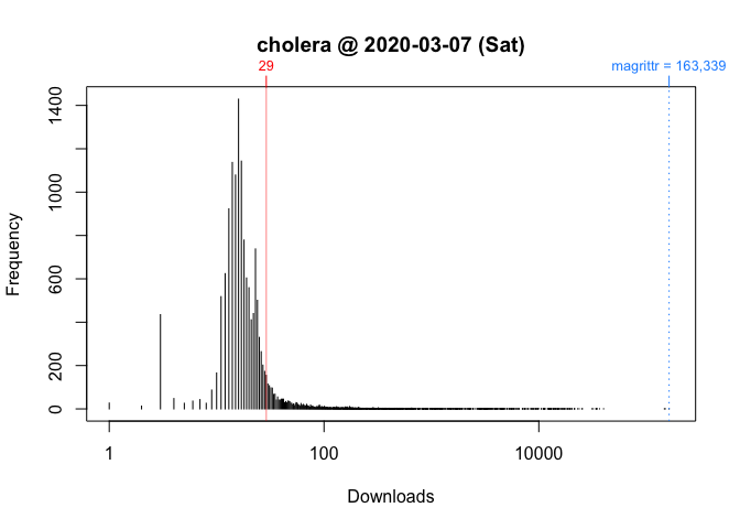
While these plots give us a better picture of where cholera is located, comparisons between Wednesday and Saturday are impressionistic at best: all we can confidently say is that the download counts for both days were greater than its respective mode.
To make interpretation and comparison easier, I use the rank percentile of a download count in place of the nominal download count. This rank percentile is a nonparametric statistic tells you the percentage of packages with fewer downloads. In other words, it gives you the location of your package relative to the location of all other packages in the distribution. Moreover, by rescaling download counts to lie on the bounded interval between 0 and 100, rank percentiles make it easier to compare packages both within and across distributions.
For example, we can compare Wednesday (“2020-03-04”) to Saturday (“2020-03-07”):
        date packages downloads            rank percentile
1 2020-03-04  cholera        38 5,556 of 18,038       67.9
packageRank(package = "cholera", date = "2020-03-04", size.filter = FALSE)
On Wednesday, we can see that cholera had 38 downloads, came in 5,556th place out of the 18,038 unique packages downloaded, and earned a spot in the 68th percentile.
        date packages downloads            rank percentile
1 2020-03-07  cholera        29 3,061 of 15,950         80
packageRank(package = "cholera", date = "2020-03-07", size.filter = FALSE)
On Saturday, we can see that cholera had 29 downloads, came in 3,061st place out of the 15,950 unique packages downloaded, and earned a spot in the 80th percentile.
So contrary to what the nominal counts tell us, one could say that the interest in cholera was actually greater on Saturday than on Wednesday.
Computing rank percentiles
To compute rank percentiles, I do the following. For each package, I tabulate the number of downloads and then compute the percentage of packages with fewer downloads. Here are the details using cholera from Wednesday as an example:
pkg.rank <- packageRank(packages = "cholera", date = "2020-03-04",
  size.filter = FALSE)

downloads <- pkg.rank$crosstab

round(100 * mean(downloads < downloads["cholera"]), 1)
[1] 67.9
To put it differently:
(pkgs.with.fewer.downloads <- sum(downloads < downloads["cholera"]))
[1] 12250
(tot.pkgs <- length(downloads))
[1] 18038
round(100 * pkgs.with.fewer.downloads / tot.pkgs, 1)
[1] 67.9
Visualizing rank percentiles
To visualize packageRank(), use plot():
plot(packageRank(packages = "cholera", date = "2020-03-04"))
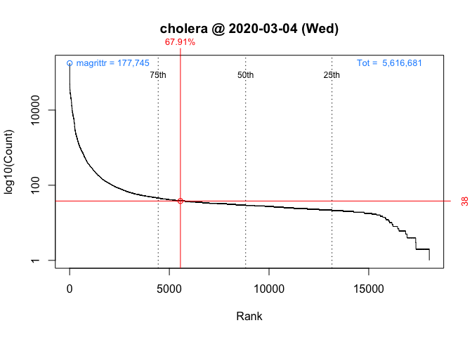
plot(packageRank(packages = "cholera", date = "2020-03-07"))
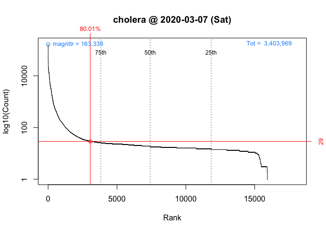
These graphs, customized to be on the same scale, plot the rank order of packages’ download counts (x-axis) against the logarithm of those counts (y-axis). It then highlights a package’s position in the distribution along with its rank percentile and download count (in red). In the background, the 75th, 50th and 25th percentiles are plotted as dotted vertical lines; the package with the most downloads, which in both cases is magrittr (in blue, top left); and the total number of downloads, 5,561,681 and 3,403,969 respectively (in blue, top right).
Computational limitations
Unlike cranlogs::cran_download(), which benefits from server-side support (i.e., download counts are “pre-computed”), packageRank() must first download the log file (upwards of 50 MB file) from the internet and then compute the rank percentiles of download counts for all observed packages (typically 15,000+ unique packages and 6 million log entries). The downloading is the real bottleneck (the computation of rank percentiles takes less than a second). This, however, is somewhat mitigated by caching the file using the memoise package.
Analytical limitations
Because of the computational limitations, anything beyond a one-day, cross-sectional comparison is “expensive”. You need to download all the desired log files (each ~50 MB). If you want to compare ranks for a week, you have to download 7 log files. If you want to compare ranks for a month, you have to download 30 odd log files.
Nevertheless, as a proof-of-concept of the potential value of computing rank percentiles over multiple time frames, the plot below compares nominal download counts with rank percentiles of cholera for the first week in March. Note that, to the chagrin of some, two independently scaled y-variables are plotted on the same graph (black for counts on the left axis, red for rank percentiles on the right).

Note that while the correlation between counts and rank percentiles is high in this example (r = 0.7), it’s not necessarily representative of the general relationship between counts and rank percentiles.
Conceptual limitations
Above, I argued that one of the virtues of the rank percentile is that it allows you to locate your package’s position relative to that of all other packages. However, one might wonder whether we may be comparing apple to oranges: just how fair or meaningful it is to compare a package like curl, an important infrastructure tool, to a package like cholera, an applied, niche application. While I believe that comparing fruit against fruit (packages against packages) can be interesting and insightful (e.g., the numerical and visual comparisons of Wednesday and Saturday), I do acknowledge that not all fruit are created equal.
This is, in fact, one of tasks I had in mind for packageRank. I wanted to create indices (e.g., Dow Jones, NASDAQ) that use download activity as a way to assess the state and health of R and its ecosystem(s). By that I mean I’d not only look at packages as a single collective entity but also as individual communities or components (i.e., the various CRAN Task Views, tidyverse, developers, end-users, etc.). To do the latter, my hope was to segment or classify packages into separate groups based on size and domain, each with its own individual index (just like various stock market indices). This effort, along with another to control for the effect of package dependencies (see below), are now on the back burner. The reason why is that I’d argue that we first need to address an inflationary bias that affects these data.
Inflationary Bias of Download Counts
Download counts are a popular way for developers to signal a package’s importance or quality, witness the frequent use of badges that advertise those numbers on repositories. To get those counts, cranlogs, which both adjustedcranlogs and packageRank among others rely on, computes the number of entries in RStudio’s download logs for a given package.
Putting aside the possibility that the logs themselves may not be representative of of R users in general1, this strategy of would be perfectly sensible. Unfortunately, three objections can be made against the assumed equivalence of download counts and the number of log entries.
The first is that package updates inflate download counts. Based on my reading of the source code and documentation, the removal of downloads due to these updates is what motivates the adjustedcranlogs package.2 However, why updates require removal, the “adjustment” is either downward or zero, is not obvious. Both package updates (existing users) and new installations (new users) would be of interest to developers (arguably both reflect interest in a package). For this reason, I’m not entirely convinced that package updates are a source of “inflation” for download counts.
The second is that package dependencies inflate download counts. The problem, in a nutshell, is that when a user chooses to download a package, they do not choose to download all the supporting, upstream packages (i.e., package dependencies) that are downloaded along with the chosen package. To me, this is the elephant-in-the-room of download count inflation (and one reason why cranlogs::cran_top_downloads() returns the usual suspects). This was one of the problems I was hoping to tackle with packageRank. What stopped me was the discovery of the next objection, which will be the focus of the rest of this post.
The third is that “invalid” log entries inflate download counts. I’ve found two “invalid” types: 1) downloads that are “too small” and 2) an overrepresentation of past versions. Downloads that are “too small” are, apparently, a software artifact. The overrepresentation of prior versions is a consequence of what appears to be efforts to mirror or download CRAN in its entirety. These efforts makes both “invalid” log entries particularly problematic. Numerically, they undermine our strategy of computing package downloads by counting logs entries. Conceptually, they lead us to overestimate the amount of interest in a package.
The inflationary effect of “invalid” log entries is variable. First, the greater a package’s “true” popularity (i.e., the number of “real” downloads), the lower the bias: essentially, the bias gets diluted as “real” downloads increase. Second, the greater the number of prior versions, the greater the bias: when all of CRAN is being downloaded, more versions mean more package downloads. Fortunately, we can minimize the bias by filtering out “small” downloads, and by filtering out or discounting prior versions.
Download logs
To understand this bias, you should look at actual download logs. You can access RStudio’s logs directly or by using packageRank::packageLog(). Below is the log for cholera for February 2, 2020:
packageLog(package = "cholera", date = "2020-02-02")
         date     time    size package version country ip_id
1  2020-02-02 03:25:16 4156216 cholera   0.7.0      US 10411
2  2020-02-02 04:24:41 4165122 cholera   0.7.0      CO  4144
3  2020-02-02 06:28:18 4165122 cholera   0.7.0      US   758
4  2020-02-02 07:57:22 4292917 cholera   0.7.0      ET  3242
5  2020-02-02 10:19:17 4147305 cholera   0.7.0      US  1047
6  2020-02-02 10:19:17   34821 cholera   0.7.0      US  1047
7  2020-02-02 10:19:17     539 cholera   0.7.0      US  1047
8  2020-02-02 10:55:22     539 cholera   0.2.1      US  1047
9  2020-02-02 10:55:22 3510325 cholera   0.2.1      US  1047
10 2020-02-02 10:55:22   65571 cholera   0.2.1      US  1047
11 2020-02-02 11:25:30 4151442 cholera   0.7.0      US  1047
12 2020-02-02 11:25:30     539 cholera   0.7.0      US  1047
13 2020-02-02 11:25:30   14701 cholera   0.7.0      US  1047
14 2020-02-02 14:23:57 4165122 cholera   0.7.0    <NA>     6
15 2020-02-02 14:51:10 4298412 cholera   0.7.0      US     2
16 2020-02-02 17:27:40 4297845 cholera   0.7.0      US     2
17 2020-02-02 18:44:10 4298744 cholera   0.7.0      US     2
18 2020-02-02 23:32:13   13247 cholera   0.6.0      GB    20
“Small” downloads
Entries 5 through 7 form the log above illustrate “small” downloads:
        date     time    size package version country ip_id
5 2020-02-02 10:19:17 4147305 cholera   0.7.0      US  1047
6 2020-02-02 10:19:17   34821 cholera   0.7.0      US  1047
7 2020-02-02 10:19:17     539 cholera   0.7.0      US  1047
Notice the differences in size: 4.1 MB, 35 kB and 539 B. On CRAN, the source and binary files of cholera are 4.0 and 4.1 MB *.tar.gz files. With “small” downloads, I’d argue that we end up over-counting the number of actual downloads.
While I’m unsure about the kB-sized entry (they seem to increasing in frequency so insights are welcome!), my current understanding is that ~500 B downloads are HTTP HEAD requests from lftp. The earliest example I’ve found goes back to “2012-10-17” (RStudio’s download logs only go back to “2012-10-01”.). I’ve also noticed that, unlike the above example, “small” downloads aren’t always paired with “complete” downloads.
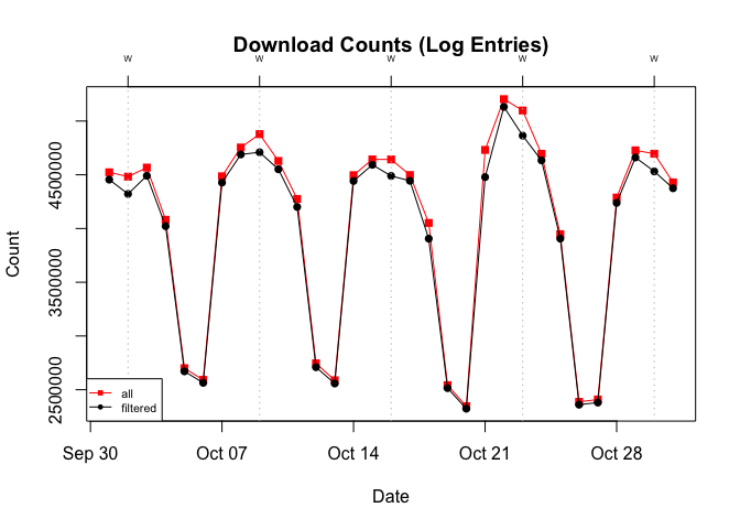
To get a sense of their frequency, I look back to October 2019 and focus on ~500 B downloads. In aggregate, these downloads account for approximately 2% of the total. While this seems modest (if 2.5 million downloads could be modest),3 I’d argue that there’s actually something lurking underneath. A closer look reveals that the difference between the total and filtered (without ~500 B entries) counts is greatest on the five Wednesdays.
To see what’s going on, I switch the unit of observation from download counts to the number of unique packages:
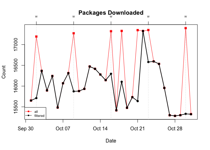
Doing so, we see that on Wednesdays (+3 additional days) the total number of unique packages downloaded tops 17,000. This is significant because it exceeds the 15,000+ active packages on CRAN (go here for the latest count). The only way to hit 17,000+ would be to include some, if not all, of the 2,000+ inactive packages. Based on this, I’d say that on those peak days virtually, if not literally, all CRAN packages (both active and inactive) were downloaded.4
Past versions
This actually understates what’s going on. It’s not just that all packages are being downloaded but that all versions of all packages are being regularly and repeatedly download. It’s these efforts, rather than downloads done for reasons of compatibility, research, or reproducibility (including the use of Docker) that lead me to argue that there’s an overrepresentation of prior versions.
As an example, see the first eight entries for cholera from the October 22, 2019 log:
packageLog(packages = "cholera", date = "2019-10-22")[1:8, ]
        date     time    size package version country  ip_id
1 2019-10-22 04:17:09 4158481 cholera   0.7.0      US 110912
2 2019-10-22 08:00:56 3797773 cholera   0.2.1      CH  24085
3 2019-10-22 08:01:06 4109048 cholera   0.3.0      UA  10526
4 2019-10-22 08:01:28 3764845 cholera   0.5.1      RU   7828
5 2019-10-22 08:01:33 4284606 cholera   0.6.5      RU  27794
6 2019-10-22 08:01:39 4275828 cholera   0.6.0      DE   6214
7 2019-10-22 08:01:43 4285678 cholera   0.4.0      RU   5721
8 2019-10-22 08:01:46 3766511 cholera   0.5.0      RU  15119
These eight entries record the download of eight different versions of cholera. A little digging with packageRank::packageHistory() reveals that the eight observed versions represent all the versions available on that day:
packageHistory("cholera")
  Package Version       Date Repository
1 cholera   0.2.1 2017-08-10    Archive
2 cholera   0.3.0 2018-01-26    Archive
3 cholera   0.4.0 2018-04-01    Archive
4 cholera   0.5.0 2018-07-16    Archive
5 cholera   0.5.1 2018-08-15    Archive
6 cholera   0.6.0 2019-03-08    Archive
7 cholera   0.6.5 2019-06-11    Archive
8 cholera   0.7.0 2019-08-28       CRAN
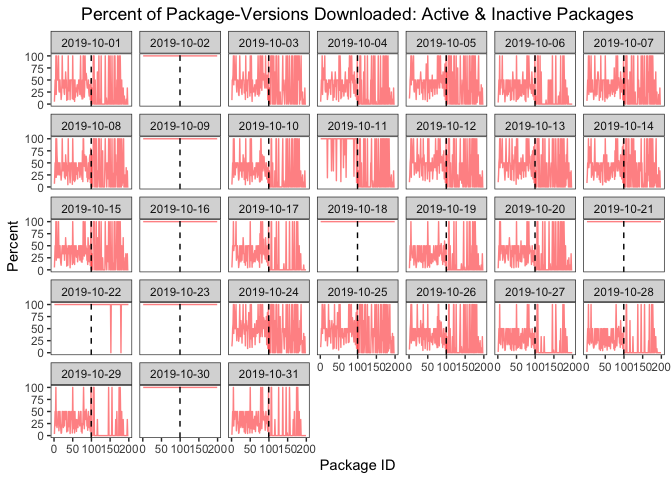
Showing that all versions of all packages are being downloaded is not as easy as showing the effect of “small” downloads. For this post, I’ll rely on a random sample of 100 active and 100 inactive packages.
The graph below plots the percent of versions downloaded for each day in October 2019 (IDs 1-100 are active packages; IDs 101-200 are inactive packages). On the five Wednesdays (+ 3 additional days), there’s a horizontal line at 100% that indicates that all versions of the packages in the sample were downloaded.5
Solutions
To minimize this bias, we could filter out “small” downloads and past versions. Filtering out 500 B downloads is simple and straightforward (packageRank() and packageLog() already include this functionality). My understanding is that there may be plans to do this in cranlogs as well. Filtering out the other “small” downloads is a bit more involved because you’d need the size of a “valid” download. Filtering out previous versions is more complicated. You’d not only need to know the current version, you’d probably also want a way to discount rather than to simply exclude previous version(s). This is especially true when a package update occurs.
Significance
Should you be worried about this inflationary bias? In general, I think the answer is yes. For most users, the goal is to estimate interest in R packages, not to estimate traffic to CRAN. To that end, “cleaner” data, which adjusts download counts to exclude “invalid” log entries should be welcome.
That said, how much you should worry depends on what you’re trying to do and which package you’re interested in. The bias works in variable, unequal fashion. It’s a function of a package’s “popularity” (i.e, the number of “valid” downloads) and the number of prior versions. A package with more “real” downloads will be less affected than one with fewer “real” downloads because the bias gets diluted (typically, “real” interest is greater than “artificial” interest). A package with more versions will be more affected because, if CRAN in its entirety is being downloaded, a package with more versions will record more downloads than one with fewer versions.
Popularity
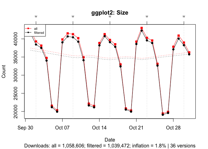
To illustrate the effect of popularity, I compare ggplot2 and cholera for October 2019. With one million plus downloads, ~500 B entries inflate the download count for ggplot2 by 2%:
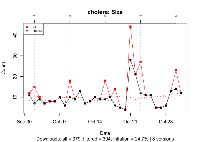
With under 400 downloads, ~500 B entries inflate the download count for cholera by 25%:
Number of versions
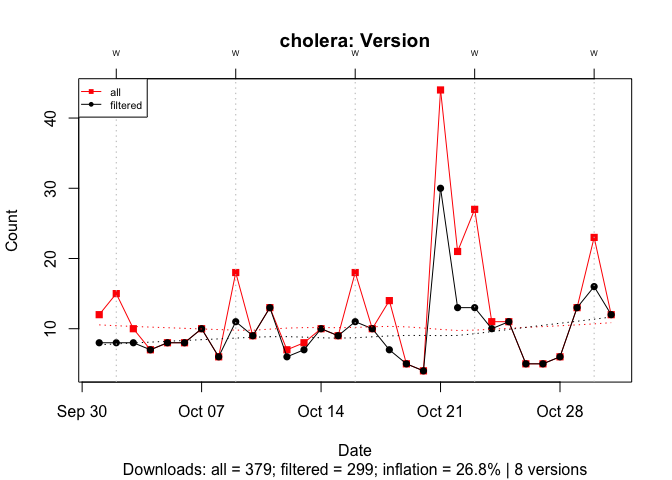
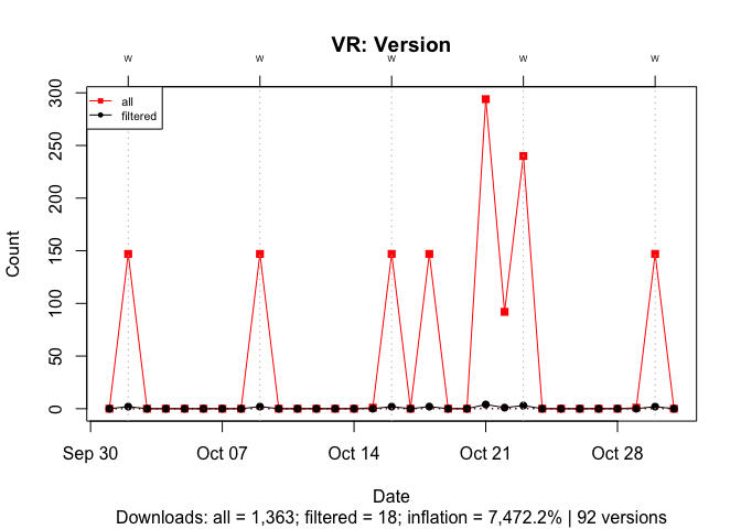
To illustrate the effect of the number of versions, I compare cholera, an active package with 8 versions, and ‘VR’, an inactive package last updated in 2009, with 92 versions. In both cases, I filter out all downloads except for those of the most recent version.
With cholera, past versions inflate the download count by 27%:
With ‘VR’, past version inflate the download count by 7,500%:
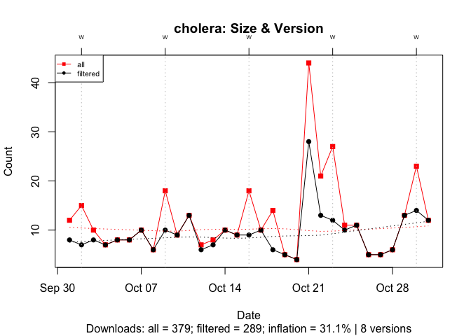
Popularity & number of versions
To illustrate the joint effect of both ~500 B downloads and previous versions, I again use cholera. Here, we see that the joint effect of both biases inflate the download count by 31%:
OLS estimate
Even though the bias is pretty mechanical and deterministic, to show that examples above are not idiosyncratic, I conclude with a back-of-the-envelope estimate of the joint, simultaneous effect of popularity (unfiltered downloads) and version count (total number of versions) on total bias (the percent change in download counts after filtering out ~500 B download and prior versions).
I use the above sample of 100 active and 100 inactive packages as the data. I fit an ordinary least squares (OLS) linear model using the base 10 logarithm for the three variables. To control for interaction between popularity and number of versions (i.e., popular packages tend to have many version; packages with many version tend to attract more downloads), I include a multiplicative term between the two variables. The results are below:
Call:
lm(formula = bias ~ popularity + versions + popularity * versions,
    data = p.data)

Residuals:
     Min       1Q   Median       3Q      Max
-0.50028 -0.12810 -0.03428  0.08074  1.09940

Coefficients:
                    Estimate Std. Error t value Pr(>|t|)
(Intercept)          2.99344    0.04769  62.768   <2e-16 ***
popularity          -0.92101    0.02471 -37.280   <2e-16 ***
versions             0.98727    0.07625  12.948   <2e-16 ***
popularity:versions  0.05918    0.03356   1.763   0.0794 .
---
Signif. codes:  0 '***' 0.001 '**' 0.01 '*' 0.05 '.' 0.1 ' ' 1

Residual standard error: 0.2188 on 195 degrees of freedom
Multiple R-squared:  0.9567,	Adjusted R-squared:  0.956
F-statistic:  1435 on 3 and 195 DF,  p-value: < 2.2e-16
The hope is that I at least get the signs right. That is, the signs of the coefficients in the fitted model (the “Estimate” column in the table above) should match the effects described above: 1) a negative sign for “popularity”, implying that greater popularity is associated with lower bias, and 2) a positive sign for “versions”, implying that a greater number of versions is associated with higher bias. For what it’s worth, the coefficients and the model itself are statistically significant at conventional levels (large t-values and small p-scores for the former; large F-statistic with a small p-score for the latter).
Conclusions
This post introduces some of the functions and features of packageRank. The aim of the package is to put package download counts into context using visualization and rank percentiles. The post also describes a systematic, positive bias that affects download counts and offers some ideas about how to minimize its effect.
The package is a work-in-progress. Please submit questions, suggestions, feature requests and problems to the comments section below or to the package’s GitHub Issues. Insights about “small” downloads are particularly welcome.