

Tables in Clinical Trials with R
2023-07-06
Chapter 1: About
1.1 Introduction
In this book we present various aspects of creating tables with the R language (R Core Team 2023) to analyze and report clinical trials data. The book was initiated by the R Consortium working group R Tables for Regulatory Submissions (RTRS). For a list of contributors to this book, see Appendix A.
The RTRS includes representation from several large pharmaceutical companies and contract research organizations. The goal of the working group is to create standards for creating tables that meet the requirements of FDA submission documents, and hence enhance the suitability of R for FDA submissions. It is part of a larger R Consortium effort to facilitate the certification and validation of R packages and tools for FDA submissions thereby allowing drug developers to submit documentation for regulatory approval using the R programming environment in conjunction with open-source packages without the need for closed and often expensive proprietary tools. For more information on the R Consortium see https://www.r-consortium.org.
1.2 Call for Contributions
The content of this book is intended to grow via community contribution, so please add your subject matter expertise to this content by cloning the Github repository of this book and making a pull request with your changes.
We welcome all contributions, including but not limited to:
- summarizing table packages
- adding new example tables
- clarifying requirements and analyses
- improving R code
In case you are new to using git and GitHub but would like to make a contribution then please write a GitHub issue and we will reach out to you to add the content.
One convenient way to get started is to:
- clone the GitHub repository of this book
- install the RStudio IDE
- Open the RStudio project in
rtrs-wg/tables-book/tables-book.Rproj - start working! See the Bookdown documentation. You can continuously preview the book with the
bookdown::serve_book()call. - once ready to share your work create a PR
- use GitHub issues to communicate with us if you have difficulties
1.3 Data Used For Examples
We use synthetic data for the examples in this book. The data is available from the random.cdisc.data R package which contains a number of datasets that follow the CDISC ADaM specifications.
remotes::install_github("insightsengineering/random.cdisc.data")The data in random.cdisc.data is completely synthetic, meaning no patient data has been used to create it. The data is also fairly basic, meaning real study data often has more signal and patterns.
data(package="random.cdisc.data")$results[, "Item"] [1] "cadab" "cadae" "cadaette" "cadcm" "caddv" "cadeg"
[7] "cadex" "cadhy" "cadlb" "cadmh" "cadpc" "cadpp"
[13] "cadqlqc" "cadqs" "cadrs" "cadsl" "cadsub" "cadtr"
[19] "cadtte" "cadvs" In this document, the prepending c stands for caches. So, for example the cached synthetic subject level dataset ADSL:
data("cadsl", package = "random.cdisc.data")
head(cadsl)
# A tibble: 6 × 55
STUDYID USUBJID SUBJID SITEID AGE AGEU SEX RACE ETHNIC COUNTRY DTHFL
<chr> <chr> <chr> <chr> <int> <fct> <fct> <fct> <fct> <fct> <fct>
1 AB12345 AB12345-CH… id-128 CHN-3 32 YEARS M ASIAN HISPA… CHN Y
2 AB12345 AB12345-CH… id-262 CHN-15 35 YEARS M BLAC… NOT H… CHN N
3 AB12345 AB12345-RU… id-378 RUS-3 30 YEARS F ASIAN NOT H… RUS N
4 AB12345 AB12345-CH… id-220 CHN-11 26 YEARS F ASIAN NOT H… CHN N
5 AB12345 AB12345-CH… id-267 CHN-7 40 YEARS M ASIAN NOT H… CHN N
6 AB12345 AB12345-CH… id-201 CHN-15 49 YEARS M ASIAN NOT H… CHN Y
# ℹ 44 more variables: INVID <chr>, INVNAM <chr>, ARM <fct>, ARMCD <fct>,
# ACTARM <fct>, ACTARMCD <fct>, TRT01P <fct>, TRT01A <fct>, TRT02P <fct>,
# TRT02A <fct>, REGION1 <fct>, STRATA1 <fct>, STRATA2 <fct>, BMRKR1 <dbl>,
# BMRKR2 <fct>, ITTFL <fct>, SAFFL <fct>, BMEASIFL <fct>, BEP01FL <fct>,
# AEWITHFL <fct>, RANDDT <date>, TRTSDTM <dttm>, TRTEDTM <dttm>,
# TRT01SDTM <dttm>, TRT01EDTM <dttm>, TRT02SDTM <dttm>, TRT02EDTM <dttm>,
# AP01SDTM <dttm>, AP01EDTM <dttm>, AP02SDTM <dttm>, AP02EDTM <dttm>, …
adsl <- cadsl1.4 Installing the R packages
At some point we may switch to renv to install the R packages used for this book. For right now you can install the packages yourself with:
install.packages(c("rtables", "tern", "gt", "remotes", "tidyverse", "bookdown",
                   "tables", "formatters", "tidytlg", "flextable"))

remotes::install_github("insightsengineering/random.cdisc.data")
remotes::install_github("insightsengineering/scda")
remotes::install_github("GSK-Biostatistics/tfrmt")
In each of the sections below, we will reset R to close to the present state at the start of the section, so readers can execute the demonstration code more or less independently of the other sections. This is done using the functions defined below. In your own documents, you wouldn’t need these resets.
References
Chapter 2: Overview of table R packages
There are many R packages available that can help with the creation of production-ready tables for clinical research. We provide here a listing of the most notable packages available for this purpose. The descriptions are meant to provide a basic overview of what each package is capable of, and, the general focus area for each. Word of warning: the list is by no means complete. There are possibly dozens of such packages, but we were selective in choosing which of those to present here (mostly in the interest of not presenting too much material, so as to not burden the reader with too many alternatives).
2.1 gt
The gt package (Iannone et al. 2023, website) provides a high-level and declarative interface for composing tables. The package contains a large variety of formatting functions for transforming cell values from an input data frame to the desired reporting values. There are options for scientific notation, percentages, localized currencies, expressing uncertainties and ranges, dates and times, etc.). The package has the ability to generate summary rows, footnotes, source notes, and structure the table with a stub and column spanners. Multiple output formats are supported with the same declarative interface (e.g., HTML, LaTeX/PDF, RTF, and Word).
The gt source code is on GitHub and the project website provides a wealth of documentation. The package is also available on CRAN.
2.2 rtables
The rtables package (Becker and Waddell 2023, website) defines a pipe-able grammar for declaring complex table structure layouts via nested splitting – in row- and column-space – and the specification of analysis functions which will calculate cell values within that structure. These pre-data table layouts are then applied to data to build the table, during which all necessary data grouping implied by the row and column splits, cell value calculation, and tabulation occurs automatically. Additional table features such as titles, footers, and referential footnotes are supported. ASCII, HTML, and PDF are supported as output formats for rendering tables.
The rtables package is available on CRAN. Its source code GitHub and documentation are also available on Github, where development of the package occurs.
rtables is also the table engine used (as wrapped by tern) in the open source TLG Catalog.
2.3 tern (+ rtables)
The tern package (Zhu et al. 2023, website) is an open sourced, opinionated TLG generation package for clinical trials. With respect to tables, tern acts as wrapper around the core rtables tabulation engine which performs two functions with respect to standard tables clinical trial tables: implementation of statistical logic, and providing convenience wrappers for common table layout patterns. In particular, tern implements and open-sources the statistical choices used by Roche ™ when constructing clinical trial tables.
The open source TLG Catalog uses tern and rtables to implement over 220 stanard clinical trial table variants across 8 table categories. The catalog includes open source-permissively licensed, runnable code for each entry.
The tern package is available on CRAN. Its source code GitHub and documentation are also available on Github, where development of the package occurs.
2.4 flextable
flextable (Gohel and Skintzos 2023, website) provides a grammar for creating and customizing tables. The following formats are supported: ‘Word’ (.docx), ‘PowerPoint’ (.pptx), ‘RTF’, ‘PDF’ ,‘HTML’ and R ‘Grid Graphics’. The syntax is the same for the user regardless of the type of output to be produced. A set of functions allows the creation, definition of cell arrangement, addition of headers or footers, formatting and definition of cell content (i.e. text and or images). The package also offers a set of high-level functions that allow, for example, tabular reporting of statistical models and the creation of complex cross tabulations.
Source code is on GitHub and a user manual is available. The package is also available on CRAN.
2.5 tfrmt
The tfrmt (Fillmore et al. 2023, website) package provides a language for defining display-related metadata and table formatting before any data is available. This package offers an intuitive interface for defining and layering standard or custom formats, to which ARD (analysis results data) is supplied. It also presents the novel ability to easily generate mock displays using metadata that will be used for the actual displays. tfrmt is built on top of the gt package, which is intended to support a variety of output formats in the future. Table features (titles, header, footnotes, etc.) as well as specific formatting (e.g. rounding, scientific notation, alignment, spacing) are supported.
The tfrmt source code is on GitHub and documentation can be found in the project website. The package is also available on CRAN.
2.6 tables
The tables package (Murdoch 2023, website) provides a formula-driven interface for computing the contents of tables and formatting them. It was inspired by SAS PROC TABULATE, but is not compatible with it.
The user computes a table object by specifying a formula, with the left-hand side giving the rows, and the right-hand side giving the columns; the formula describes the summary functions to apply and how to organize them. The objects can be subsetted or combined using matrix-like operations. Tables can be rendered in plain text, LaTeX code to appear in a PDF document, or HTML code for a web document.
The package is on CRAN. Source is maintained on Github at https://github.com/dmurdoch/tables/. Vignettes in the package serve as a user manual; browse them at https://dmurdoch.github.io/tables/, or install the package, then run browseVignettes(package = "tables").
2.7 tidytlg
The tidytlg package (Masel et al. 2023, website) provides a framework for creating tables, listings, and graphs (TLGs) using Tidyverse (Wickham et al. 2019). It offers a suite of analysis functions to summarize descriptive statistics (univariate statistics and counts or percentages) for table creation and a function to convert analysis results to rtf/html outputs. For graphic output, tidytlg can integrate plot objects created by ggplot2 or a png file with titles and footnotes to produce rtf/html output.
tidytlg source code and documentation are on Github.
References
Chapter 3: Formatting and Rendering Tables
Table generation usually is a two step process
- Derive the cell value and tabulate them.
- Create the final table output, save it to a file to be shared with collaborators.
Chapter Commonly Used Tables focuses on the work involved in step 1. In this chapter we discuss the various aspects of creating the final output that is commonly stored in a file with a particular file format (pdf, txt, html, docx or rtf).
3.1 Title & Footnotes
Commonly rendered tables that are reported to the health authorities have titles and footnotes with information such as:
- what is summarized in the table
- database lock date
- patient sub-population
- notes by study team
- notes regarding statistical algorithms chosen
- provenance information including path to program and when the table was created
Often footnotes include cell references.
3.1.1 gt
The gt package lets you add a title and even a subtitle and preheader lines (for RTF) with its tab_header() function. In the following example, we create some sample_data and feed that into the gt() function. We can automatically create a table stub (for row labels) and row groups with the rowname_col and groupname_col arguments of gt().
resetSession()
library(gt)

sample_data <-
  dplyr::tibble(
    label = c("n", "Mean (SD)", "Median", "Min - Max", "F", "M", "U", "UNDIFFERENTIATED"),
    `val_A: Drug X` = c(134, 33.8, 33, NA, 79, 51, 3, 1),
    `val_B: Placebo` = c(134, 35.4, 35, NA, 77, 55, 2, 0),
    `val_C: Combination` = c(132, 35.4, 35, NA, 66, 60, 4, 2),
    category = c(rep("Age (Years)", 4), rep("Sex, n (%)", 4))
  )

gt_tbl <-
  gt(
    sample_data,
    rowname_col = "label",
    groupname_col = "category"
  ) |>
  tab_header(
    title = "x.x: Study Subject Data",
    subtitle = md(
      "x.x.x: Demographic Characteristics  \n Table x.x.x.x: Demographic
      Characteristics - Full Analysis Set"
    ),
    preheader = c("Protocol: XXXXX", "Cutoff date: DDMMYYYY")
  ) |>
  tab_source_note("Source: ADSL DDMMYYYY hh:mm; Listing x.xx; SDTM package: DDMMYYYY") |>
  sub_missing(missing_text = "") |>
  tab_options(
    page.orientation = "landscape",
    page.numbering = TRUE,
    page.header.use_tbl_headings = TRUE,
    page.footer.use_tbl_notes = TRUE
  )

gt_tbl| x.x: Study Subject Data | |||
| x.x.x: Demographic Characteristics Table x.x.x.x: Demographic Characteristics – Full Analysis Set |
|||
| val_A: Drug X | val_B: Placebo | val_C: Combination | |
|---|---|---|---|
| Age (Years) | |||
| n | 134.0 | 134.0 | 132.0 |
| Mean (SD) | 33.8 | 35.4 | 35.4 |
| Median | 33.0 | 35.0 | 35.0 |
| Min – Max | |||
| Sex, n (%) | |||
| F | 79.0 | 77.0 | 66.0 |
| M | 51.0 | 55.0 | 60.0 |
| U | 3.0 | 2.0 | 4.0 |
| UNDIFFERENTIATED | 1.0 | 0.0 | 2.0 |
| Source: ADSL DDMMYYYY hh:mm; Listing x.xx; SDTM package: DDMMYYYY | |||
The above example contains the use of the tab_source_note() function. You can create as many source notes in the table footer as you need, and they typically describe the data table as a whole (i.e., not pointing to anything specific). For that, you can use footnotes and target cells that require additional explanation. Here’s an example of that using tab_footnote():
gt_tbl |>
  tab_footnote(
    footnote = "This is the combination of the two.",
    locations = cells_column_labels(columns = `val_C: Combination`)
  ) |>
  tab_footnote(
    footnote = "These values are the same.",
    locations = cells_body(
      columns = matches("_A|_B"), rows = "n"
      )
)| x.x: Study Subject Data | |||
| x.x.x: Demographic Characteristics Table x.x.x.x: Demographic Characteristics – Full Analysis Set |
|||
| val_A: Drug X | val_B: Placebo | val_C: Combination1 | |
|---|---|---|---|
| Age (Years) | |||
| n | 2 134.0 | 2 134.0 | 132.0 |
| Mean (SD) | 33.8 | 35.4 | 35.4 |
| Median | 33.0 | 35.0 | 35.0 |
| Min – Max | |||
| Sex, n (%) | |||
| F | 79.0 | 77.0 | 66.0 |
| M | 51.0 | 55.0 | 60.0 |
| U | 3.0 | 2.0 | 4.0 |
| UNDIFFERENTIATED | 1.0 | 0.0 | 2.0 |
| Source: ADSL DDMMYYYY hh:mm; Listing x.xx; SDTM package: DDMMYYYY | |||
| 1 This is the combination of the two. | |||
| 2 These values are the same. | |||
The tab_footnote() function allows for footnotes to be placed anywhere in the table (using the cells_*() helper functions for targeting). Targeting columns, rows, or other locations can be done with Tidyselect-style helper functions (e.g., matches(), starts_with(), etc.), ID values, or indices.
As a final note on the first example, we can specify certain page.* options that make RTF output ideal for regulatory filing purposes. The options employed above in the tab_options() call ensure that pages are in landscape orientation, page numbering for each table is activated, and that page header and footer are used for the table’s headings and footer elements.
3.1.2 rtables
The basic_table() function in rtables has the arguments titles, subtitles, main_footer, prov_footer to add titles and footnotes to tables. rtables also supports referential footnotes.
So for example a basic demographics table created with rtables via tern with title and footnotes would look as follows:
resetSession()
library(rtables)

lyt <- basic_table(
  title = "Demographic Table - All Patients",
  subtitles = c("Cutoff Date: June 01, 2022", "Arm B received a placebo."),
  main_footer = c("Missing data is omitted.")
) |>
  split_cols_by("ARM") |>
  analyze(c("AGE", "SEX"))

build_table(lyt, adsl)
Demographic Table - All Patients
Cutoff Date: June 01, 2022
Arm B received a placebo.
————————————————————————————————————————————————
A: Drug X B: Placebo C: Combination
————————————————————————————————————————————————
AGE
Mean 33.77 35.43 35.43
SEX
F 79 82 70
M 55 52 62
————————————————————————————————————————————————
Missing data is omitted.3.1.3 flextable
Titles and notes can be added and formatted with the flextable package. It is possible to add them in the header and in the footer. Several methods are possible but for most needs, the add_header_lines() and add_footer_lines() functions will be the easiest to use.
Let’s create first a flextable from an aggregation that will be used to illustrate the features.
resetSession()
library(flextable)
library(dplyr)

z <- adsl |>
  group_by(ARM, SEX) |>
  summarise(avg = mean(AGE), sd = sd(AGE)) |>
  tabulator(rows = "SEX", columns = "ARM",
    Y = as_paragraph(avg, " (", sd, ")")) |>
  as_flextable()
z|
SEX |
|
A: Drug X |
|
B: Placebo |
|
C: Combination |
|---|---|---|---|---|---|---|
|
F |
|
32.8 (6.1) |
|
34.2 (7.0) |
|
35.2 (7.4) |
|
M |
|
35.2 (7.0) |
|
37.3 (8.9) |
|
35.7 (8.2) |
The following shows how to add titles or notes:
z |>
  add_header_lines("hello world") |>
add_footer_lines("bye bye world")|
hello world |
||||||
|---|---|---|---|---|---|---|
|
SEX |
|
A: Drug X |
|
B: Placebo |
|
C: Combination |
|
F |
|
32.8 (6.1) |
|
34.2 (7.0) |
|
35.2 (7.4) |
|
M |
|
35.2 (7.0) |
|
37.3 (8.9) |
|
35.7 (8.2) |
|
bye bye world |
||||||
For Word output, users can prepend a table number that will auto-incremente.
docx_file <- "reports/flextable-title-01.docx"
ft <- add_header_lines(z, "hello world") |>
  prepend_chunks(
    i = 1, j = 1, part = "header",
    as_chunk("Table "), as_word_field("SEQ tab \u005C* Arabic"),
    as_chunk(": ")) |>
  add_footer_lines("bye bye world") |>
  theme_vanilla()
save_as_docx(ft, ft, path = docx_file)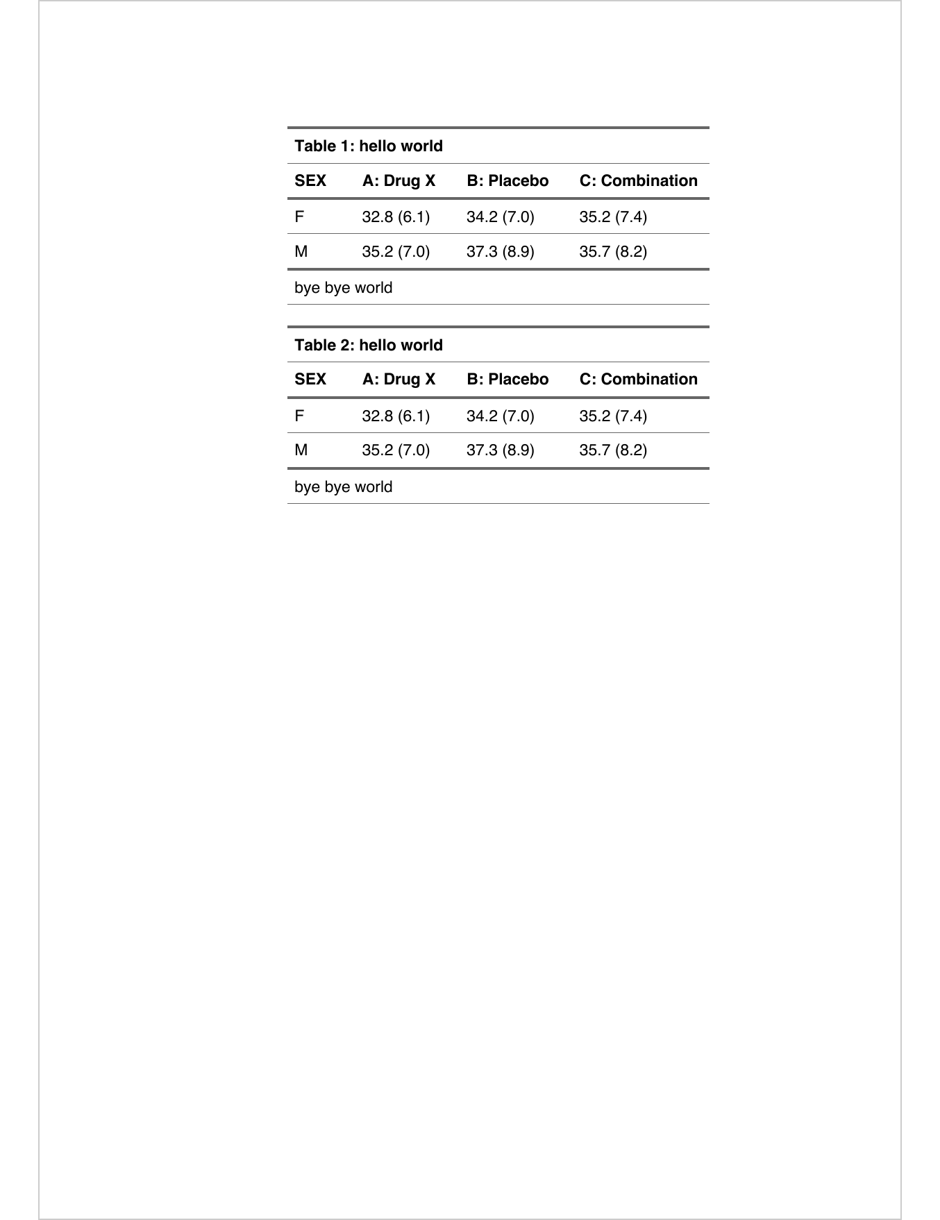
Footnotes are also available in flextable with function footnote(). The function lets users add footnotes and references to it on the table.
footnote(z, i = c(1, 2, 2), j = c(1, 5, 7),
value = as_paragraph("hello world"), ref_symbols = "(1)")|
SEX |
|
A: Drug X |
|
B: Placebo |
|
C: Combination |
|---|---|---|---|---|---|---|
|
F(1) |
|
32.8 (6.1) |
|
34.2 (7.0) |
|
35.2 (7.4) |
|
M |
|
35.2 (7.0) |
|
37.3 (8.9)(1) |
|
35.7 (8.2)(1) |
|
(1)hello world |
||||||
3.1.4 tfrmt
The tfrmt() function in the tfrmt package includes the arguments title and subtitle to add titles. Within the footnote_plan() function, the user can nest multiple footnote_structures to add footnotes with superscript reference symbols on groups, columns or labels.
To demonstrate, this example will create a mock demographics table:
resetSession()
library(tfrmt)
library(dplyr)
library(tidyr)

# Create mock data
df <- crossing(group = c("AGE", "SEX"),
               label = c("label 1", "label 2"),
               column = c("Drug X", "Placebo", "Combination"),
               param = c("count", "percent"))

# Create specification
tfrmt_spec <- tfrmt(
  # Add titles
  title = "Demographic Table - All Patients",
  subtitle = "Cutoff Date: June 01, 2022. Arm B received a placebo.",

  # Specify table features
  group = group,
  label = label,
  column = column,
  param = param,
  row_grp_plan = row_grp_plan(
    row_grp_structure(group_val = ".default",
                      element_block(post_space = "   ")) ),

  # Define cell formatting
  body_plan = body_plan(
    frmt_structure(group_val = ".default", label_val = ".default",
                   frmt_combine("{count} ({percent})",
                                count = frmt("xx"),
                                percent = frmt("xx.x")))),

  # Add footnotes here
  footnote_plan = footnote_plan(
    footnote_structure(footnote_text = "Footnote about column", column_val = "Combination"),
    footnote_structure(footnote_text = "Footnote about group", group_val = "AGE"),
    marks = "numbers"),

)

print_mock_gt(tfrmt_spec, df)| Demographic Table – All Patients | |||
| Cutoff Date: June 01, 2022. Arm B received a placebo. | |||
| Combination1 | Drug X | Placebo | |
|---|---|---|---|
| AGE2 | |||
| label 1 | xx (xx.x) | xx (xx.x) | xx (xx.x) |
| label 2 | xx (xx.x) | xx (xx.x) | xx (xx.x) |
| SEX | |||
| label 1 | xx (xx.x) | xx (xx.x) | xx (xx.x) |
| label 2 | xx (xx.x) | xx (xx.x) | xx (xx.x) |
| 1 Footnote about column | |||
| 2 Footnote about group | |||
See this vignette for more details on footnotes: link to website
3.1.5 tables
The tables package concentrates on the table itself. The titles are generally written as part of the surrounding document. Footnotes would be added after constructing the table by modifying individual entries.
Alternatively for HTML output, only the footnote markers need to be added by modifying entries, and then the footnotes can be applied by using toHTML(tab, options = list(doFooter = TRUE, HTMLfooter = HTMLfootnotes(...)).
resetSession()
adsl <- cadsl

library(tables)
table_options(doCSS = TRUE)

sd_in_parens <- function(x) sprintf("(%.1f)", sd(x))

tab <- tabular(SEX ~ Heading()*ARM*
                     Heading()*AGE*
                     Heading()*(mean + sd_in_parens),
               data = adsl)

rowLabels(tab)[1,1] <- paste(rowLabels(tab)[1,1], "<sup>a</sup>")
tab[2,2] <- sprintf("%s%s", tab[2,2], "<sup>b</sup>")
tab[2,3] <- sprintf("%.2f%s", tab[2,3], "<sup>b</sup>")

footnotes <- HTMLfootnotes(tab, a = "This is a label footnote.",
                                b = "These are cell footnotes.")
toHTML(tab, options = list(HTMLfooter = footnotes,
doFooter = TRUE))| SEX | A: Drug X | B: Placebo | C: Combination | |||
|---|---|---|---|---|---|---|
| aThis is a label footnote. bThese are cell footnotes. |
||||||
| F a | 32.76 | (6.1) | 34.24 | (7.0) | 35.20 | (7.4) |
| M | 35.22 | (7.0)b | 37.31b | (8.9) | 35.69 | (8.2) |
3.1.6 tidytlg
The gentlg() function in the tidytlg package includes the title argument for adding title and the footers argument for adding footnotes to the table output. Users can include a vector of character strings for multiple lines of footnotes (please see an example below). At the bottom line of the footnotes, the file name of the table and the path of the table program along with the datetime stamp are automatically created.
resetSession()
library(dplyr)
library(tidytlg)

adsl <- formatters::ex_adsl

# create analysis set row
t1 <- freq(adsl,
           rowvar = "ITTFL",
           colvar = "ARM",
           statlist = statlist("n"),
           subset = ITTFL == "Y",
           rowtext = "Analysis set: ITT")

# create univariate stats for age
t2 <- univar(adsl,
               rowvar = "AGE",
               colvar = "ARM",
               statlist = statlist(c("N", "MEANSD", "MEDIAN", "RANGE", "IQRANGE")),
               row_header = "Age (years)",
               decimal = 0)

tbl <- bind_table(t1, t2)

# assign table id
tblid <- "Table01"

# output the analysis results
gentlg(huxme       = tbl,
       format      = "HTML",
       print.hux = FALSE,
       file        = tblid,
       orientation = "portrait",
       title = "Demographic and Baseline Characteristics; Intent-to-treat Analysis Set",
       footers = c("Key: IQ = Interquartile","Note: N reflects non-missing values"),
colheader = c("","A: Drug X","B: Placebo","C: Combination"))|
Table01: Demographic and Baseline Characteristics; Intent-to-treat Analysis Set
|
|||
|
A: Drug X
|
B: Placebo
|
C: Combination
|
|
|---|---|---|---|
|
Analysis set: ITT
|
134 | 134 | 132 |
|
Age (years)
|
|||
|
N
|
134 | 134 | 132 |
|
Mean (SD)
|
33.8 (6.55) | 35.4 (7.90) | 35.4 (7.72) |
|
Median
|
33.0 | 35.0 | 35.0 |
|
Range
|
(21; 50) | (21; 62) | (20; 69) |
|
IQ range
|
(28.0; 39.0) | (30.0; 40.0) | (30.0; 40.0) |
|
Key: IQ = Interquartile
|
|||
| Note: N reflects non-missing values | |||
|
[table01.html][/home/runner/work/_temp/75195cf9-5534-4d13-ba4e-dde001586365] 06JUL2023, 23:51
|
|||
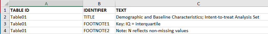
To programmatically incorporate titles and footnotes into each table program, users can create an excel file called titles.xls (see below snapshot) with the columns of "TABLE ID","IDENTIFIER","TEXT". In the gentlg() function call, users just need to provide the argument of title_file for specifying the location of titles.xls. Then the title and footnotes corresponding to the table ID will be automatically included in the table output. Users need to make sure the correct table ID is used for the file argument of the gentlg() function call.
gentlg(huxme       = tbl,
       format      = "HTML",
       print.hux = FALSE,
       file        = tblid,
       orientation = "portrait",
       title_file = system.file("extdata/titles.xls", package = "tidytlg"),
       colheader = c("","A: Drug X","B: Placebo","C: Combination"))
3.2 Captions
A caption is a single paragraph of text describing the table. Captions are often used because they allow you to cross-reference tables or list them in a ‘list of tables’ with the corresponding page numbers.
3.2.1 flextable
The set_caption() function in flextable is the recommended way to add captions.
resetSession()
library(flextable)

flextable(head(cars)) |>
  set_caption(
    caption = "a caption",
autonum = officer::run_autonum(seq_id = "tab", bkm = "flextable-label"))|
speed |
dist |
|---|---|
|
4 |
2 |
|
4 |
10 |
|
7 |
4 |
|
7 |
22 |
|
8 |
16 |
|
9 |
10 |
In bookdown, use the syntax \@ref(tab:flextable-label) to create a linked reference to the table. Here is an example of a reference: 3.2.
With Quarto, the R chunk code should be transformed as:
#| label: tbl-flextable-label
#| tbl-cap: a caption
flextable(head(cars))
3.2.2 tables
As with titles, captions would be added as part of the surrounding document rather than part of the table object.
3.3 Pagination
Historically tables have been printed to paper for submissions. Hence large tables that would not fit onto a single printed page (e.g. letter & portrait) would have to be split into multiple tables that can be printed to the preferred page size. This process of splitting the table is called pagination of tables.
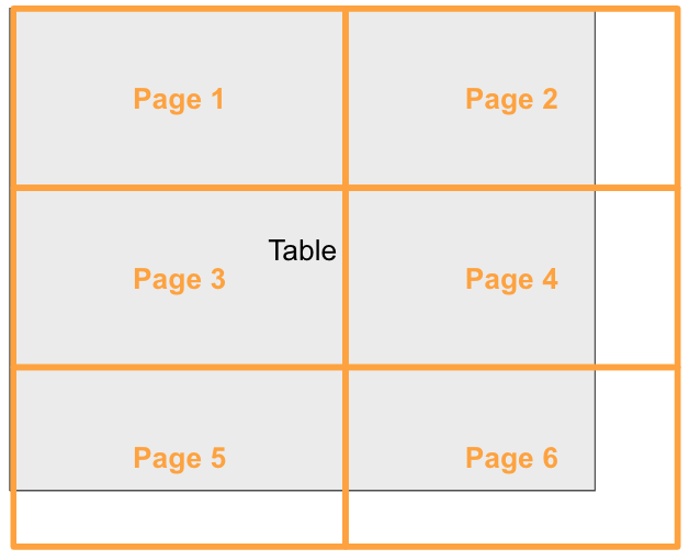
Illustration of a table being paginated in both horizontal and vertical directions
Pagination of complex structured tables is complicated by the fact that some rows of such tables require contextual information – e.g., any group labels or summaries they fall under – to be fully understood. This means that any such context must be repeated after a page break for that page to be understood in isolation.
3.3.1 rtables
rtables supports context-preserving pagination in both the horizontal and vertical directions (via the interface provided by formatters) via calling paginate_table() directly, and within the export_as_* rendering functions. Users specify page dimensions (in either inches, or lines long and characters wide) and font information and the pagination and export machinery paginates the table such that each portion will fit fully on its page when rendered as text, including title, footer, and referential footnote materials.
For vertical pagination, summary rows (whether label rows, or so-called content rows containing summary values) are repeated after page breaks to preserve context on the following page. We see this in action below when pagination occurs within the strtata B – ASIAN facet of the the following table
resetSession()
library(rtables)

lyt <- basic_table(title = "main title", subtitles = "subtitle", main_footer = "main footer", prov_footer = "provenance footer") |>
  split_cols_by("ARM") |>
  split_cols_by("SEX", split_fun = keep_split_levels(c("F", "M"))) |>
  split_rows_by("STRATA1", split_fun = keep_split_levels(c("A", "B"))) |>
  split_rows_by("RACE", split_fun = keep_split_levels(c("ASIAN", "WHITE"))) |>
  summarize_row_groups() |>
  analyze("AGE", afun = function(x, ...) in_rows("mean (sd)" = rcell(c(mean(x), sd(x)), format = "xx.x (xx.x)"),
                                                 "range" = rcell(range(x), format = "xx.x - xx.x")))

tbl <- build_table(lyt, ex_adsl)
tbl
main title
subtitle
—————————————————————————————————————————————————————————————————————————————————————————————————
A: Drug X B: Placebo C: Combination
F M F M F M
—————————————————————————————————————————————————————————————————————————————————————————————————
A
ASIAN 11 (13.9%) 10 (19.6%) 14 (18.2%) 10 (18.2%) 11 (16.7%) 7 (11.7%)
mean (sd) 29.0 (3.9) 35.0 (6.1) 31.1 (5.5) 40.9 (10.3) 33.7 (4.0) 37.0 (5.9)
range 24.0 - 35.0 28.0 - 43.0 23.0 - 46.0 27.0 - 62.0 28.0 - 40.0 28.0 - 47.0
WHITE 5 (6.3%) 3 (5.9%) 3 (3.9%) 3 (5.5%) 3 (4.5%) 5 (8.3%)
mean (sd) 34.4 (2.9) 35.3 (8.5) 33.7 (2.9) 38.7 (10.3) 29.7 (6.1) 32.2 (7.7)
range 30.0 - 37.0 29.0 - 45.0 32.0 - 37.0 30.0 - 50.0 23.0 - 35.0 25.0 - 45.0
B
ASIAN 11 (13.9%) 9 (17.6%) 15 (19.5%) 7 (12.7%) 11 (16.7%) 14 (23.3%)
mean (sd) 29.5 (5.7) 35.3 (7.1) 38.7 (10.0) 37.6 (10.6) 41.5 (9.6) 36.1 (7.5)
range 23.0 - 40.0 27.0 - 48.0 26.0 - 58.0 26.0 - 58.0 32.0 - 64.0 25.0 - 48.0
WHITE 5 (6.3%) 4 (7.8%) 8 (10.4%) 4 (7.3%) 5 (7.6%) 2 (3.3%)
mean (sd) 35.0 (3.4) 39.0 (11.2) 32.2 (5.3) 33.0 (9.8) 33.4 (6.5) 29.0 (4.2)
range 31.0 - 39.0 24.0 - 48.0 26.0 - 42.0 21.0 - 42.0 28.0 - 44.0 26.0 - 32.0
—————————————————————————————————————————————————————————————————————————————————————————————————
main footer
provenance footerpaginate_table(), then, breaks our table into subtables – including repeated context where appropriate – which will fit on physical pages (we use 5.2 x 3.5 inch “pages” for illustrative purposes here):
paginate_table(tbl, pg_width = 5.2, pg_height = 3.5, min_siblings = 0)[[1]]
main title
subtitle
———————————————————————————————————————————————————————
A: Drug X B: Placebo
F M F
———————————————————————————————————————————————————————
A
ASIAN 11 (13.9%) 10 (19.6%) 14 (18.2%)
mean (sd) 29.0 (3.9) 35.0 (6.1) 31.1 (5.5)
range 24.0 - 35.0 28.0 - 43.0 23.0 - 46.0
WHITE 5 (6.3%) 3 (5.9%) 3 (3.9%)
mean (sd) 34.4 (2.9) 35.3 (8.5) 33.7 (2.9)
range 30.0 - 37.0 29.0 - 45.0 32.0 - 37.0
B
ASIAN 11 (13.9%) 9 (17.6%) 15 (19.5%)
mean (sd) 29.5 (5.7) 35.3 (7.1) 38.7 (10.0)
———————————————————————————————————————————————————————
main footer
provenance footer
[[2]]
main title
subtitle
———————————————————————————————————————————————————————
B: Placebo C: Combination
M F M
———————————————————————————————————————————————————————
A
ASIAN 10 (18.2%) 11 (16.7%) 7 (11.7%)
mean (sd) 40.9 (10.3) 33.7 (4.0) 37.0 (5.9)
range 27.0 - 62.0 28.0 - 40.0 28.0 - 47.0
WHITE 3 (5.5%) 3 (4.5%) 5 (8.3%)
mean (sd) 38.7 (10.3) 29.7 (6.1) 32.2 (7.7)
range 30.0 - 50.0 23.0 - 35.0 25.0 - 45.0
B
ASIAN 7 (12.7%) 11 (16.7%) 14 (23.3%)
mean (sd) 37.6 (10.6) 41.5 (9.6) 36.1 (7.5)
———————————————————————————————————————————————————————
main footer
provenance footer
[[3]]
main title
subtitle
———————————————————————————————————————————————————————
A: Drug X B: Placebo
F M F
———————————————————————————————————————————————————————
B
ASIAN 11 (13.9%) 9 (17.6%) 15 (19.5%)
range 23.0 - 40.0 27.0 - 48.0 26.0 - 58.0
WHITE 5 (6.3%) 4 (7.8%) 8 (10.4%)
mean (sd) 35.0 (3.4) 39.0 (11.2) 32.2 (5.3)
range 31.0 - 39.0 24.0 - 48.0 26.0 - 42.0
———————————————————————————————————————————————————————
main footer
provenance footer
[[4]]
main title
subtitle
———————————————————————————————————————————————————————
B: Placebo C: Combination
M F M
———————————————————————————————————————————————————————
B
ASIAN 7 (12.7%) 11 (16.7%) 14 (23.3%)
range 26.0 - 58.0 32.0 - 64.0 25.0 - 48.0
WHITE 4 (7.3%) 5 (7.6%) 2 (3.3%)
mean (sd) 33.0 (9.8) 33.4 (6.5) 29.0 (4.2)
range 21.0 - 42.0 28.0 - 44.0 26.0 - 32.0
———————————————————————————————————————————————————————
main footer
provenance footerrtables also supports page-by splits in its layouting framework, which declares that – regardless of rendering dimensions – pagination should occur between distinct levels of a variable. Each of these “pagination sections” have an additional title specific to the level, and are independently paginated for dimension as needed.
lyt2 <- basic_table(title = "main title", subtitles = "subtitle", main_footer = "main footer", prov_footer = "provenance footer") |>
  split_cols_by("ARM") |>
  split_rows_by("STRATA1", split_fun = keep_split_levels(c("A", "B")), page_by = TRUE, page_prefix = "Stratum") |>
  split_rows_by("RACE", split_fun = keep_split_levels(c("ASIAN", "WHITE"))) |>
  summarize_row_groups() |>
  analyze("AGE", afun = function(x, ...) in_rows("mean (sd)" = rcell(c(mean(x), sd(x)), format = "xx.x (xx.x)"),
                                                 "range" = rcell(range(x), format = "xx.x - xx.x")))

tbl2 <- build_table(lyt2, ex_adsl)

paginate_table(tbl2, lpp = 16)
$A1
main title
subtitle
Stratum: A
————————————————————————————————————————————————————————
A: Drug X B: Placebo C: Combination
————————————————————————————————————————————————————————
ASIAN 22 (16.4%) 24 (17.9%) 19 (14.4%)
mean (sd) 31.9 (5.7) 35.2 (9.1) 35.2 (4.8)
range 24.0 - 43.0 23.0 - 62.0 28.0 - 47.0
————————————————————————————————————————————————————————
main footer
provenance footer
$A2
main title
subtitle
Stratum: A
————————————————————————————————————————————————————————
A: Drug X B: Placebo C: Combination
————————————————————————————————————————————————————————
WHITE 8 (6.0%) 7 (5.2%) 8 (6.1%)
mean (sd) 34.8 (5.1) 34.9 (7.5) 31.2 (6.8)
range 29.0 - 45.0 27.0 - 50.0 23.0 - 45.0
————————————————————————————————————————————————————————
main footer
provenance footer
$B1
main title
subtitle
Stratum: B
————————————————————————————————————————————————————————
A: Drug X B: Placebo C: Combination
————————————————————————————————————————————————————————
ASIAN 20 (14.9%) 23 (17.2%) 25 (18.9%)
mean (sd) 32.1 (6.9) 38.2 (9.8) 38.4 (8.8)
range 23.0 - 48.0 26.0 - 58.0 25.0 - 64.0
————————————————————————————————————————————————————————
main footer
provenance footer
$B2
main title
subtitle
Stratum: B
————————————————————————————————————————————————————————
A: Drug X B: Placebo C: Combination
————————————————————————————————————————————————————————
WHITE 10 (7.5%) 12 (9.0%) 7 (5.3%)
mean (sd) 35.9 (7.6) 32.5 (6.7) 32.1 (6.0)
range 24.0 - 48.0 21.0 - 42.0 26.0 - 44.0
————————————————————————————————————————————————————————
main footer
provenance footer3.3.2 flextable
The pagination of flextable objects let user control their position in relation to page breaks. It can prevent breaks between tables rows of a same group.
Function paginate() let you define this pagination, this feature is only available for RTF and Word outputs; see the documentation about pagination.
3.3.3 tables
Tables that span multiple pages are supported in PDF output using the LaTeX longtable package, specified when converting to LaTeX.
3.4 Rendering Tables
The choice of output format is often dictated by your company’s processes to include the tables in a report. The packages discussed in this book vary in regard to which output formats are supported natively. The following table shows the current output capabilities for each package.
| ASCII | HTML | .docx | RTF | .pptx | grid | ||
|---|---|---|---|---|---|---|---|
| flextable | ✓ | ✓ | ✓ | ✓ | ✓ | ✓ | |
| gt | ✓ | ✓ | ✓ | ✓ | |||
| rtables | ✓ | ✓ | ✓ | ✓ | ✓ | ✓ | ✓ |
| tables | ✓ | ✓ | ✓ | ||||
| tfrmt | ✓ | ✓ | ✓ | ✓ | |||
| tidytlg | ✓ | ✓ |
If the format you need is not supported by the package you would like to use, there are still options. For example, tables produced in rtables and tables can be converted to flextable objects, giving access to the other output formats. Pandoc (MacFarlane 2023) is another option: it can convert documents between a wide range of document formats.
References
Chapter 4 Commonly Used Tables
4.1 Demographic Tables
4.1.1 rtables
Using rtables only:
resetSession()
library(rtables)

a_demo_num <- function(x) {
    in_rows(n = length(x),
            "Mean (SD)" = rcell(c(mean(x, na.rm = TRUE),
                                  sd(x, na.rm=TRUE)), format = "xx.x (xx.x)"),
            "Median" = median(x,na.rm = TRUE),
            "Min - Max" = rcell(range(x, na.rm = TRUE), format = "xx.x - xx.x"))
}

a_demo_fac <- function(x) {
    in_rows(.list = c(c(n = length(x)), table(x)))
}

lyt <- basic_table(title = "x.x: Study Subject Data",
                   subtitles= c("x.x.x: Demographic Characteristics",
                                "Table x.x.x.x: Demographic Characteristics - Full Analysis Set"),
                   prov_footer = "Source: ADSL DDMMYYYY hh:mm; Listing x.xx; SDTM package: DDMMYYYY") |>
  split_cols_by("ARM") |>
  analyze(c("AGE", "SEX", "COUNTRY"), afun = list(AGE = a_demo_num, SEX = a_demo_fac,
                                                  COUNTRY = a_demo_fac))

build_table(lyt, ex_adsl)
x.x: Study Subject Data
x.x.x: Demographic Characteristics
Table x.x.x.x: Demographic Characteristics - Full Analysis Set
———————————————————————————————————————————————————————————————
A: Drug X B: Placebo C: Combination
———————————————————————————————————————————————————————————————
AGE
n 134 134 132
Mean (SD) 33.8 (6.6) 35.4 (7.9) 35.4 (7.7)
Median 33 35 35
Min - Max 21.0 - 50.0 21.0 - 62.0 20.0 - 69.0
SEX
n 134 134 132
F 79 77 66
M 51 55 60
U 3 2 4
UNDIFFERENTIATED 1 0 2
COUNTRY
n 134 134 132
CHN 74 81 64
USA 10 13 17
BRA 13 7 10
PAK 12 9 10
NGA 8 7 11
RUS 5 8 6
JPN 5 4 9
GBR 4 3 2
CAN 3 2 3
CHE 0 0 0
———————————————————————————————————————————————————————————————
Source: ADSL DDMMYYYY hh:mm; Listing x.xx; SDTM package: DDMMYYYY4.1.2 tern (+ rtables)
resetSession()
library(tern)
lyt <- basic_table(title = "x.x: Study Subject Data",
                   subtitles= c("x.x.x: Demographic Characteristics",
                                "Table x.x.x.x: Demographic Characteristics - Full Analysis Set"),
                   prov_footer = "Source: ADSL DDMMYYYY hh:mm; Listing x.xx; SDTM package: DDMMYYYY") |>
  split_cols_by("ARM") |>
  summarize_vars(c("AGE", "SEX", "COUNTRY"))

build_table(lyt, ex_adsl)
x.x: Study Subject Data
x.x.x: Demographic Characteristics
Table x.x.x.x: Demographic Characteristics - Full Analysis Set
———————————————————————————————————————————————————————————————
A: Drug X B: Placebo C: Combination
———————————————————————————————————————————————————————————————
AGE
n 134 134 132
Mean (SD) 33.8 (6.6) 35.4 (7.9) 35.4 (7.7)
Median 33.0 35.0 35.0
Min - Max 21.0 - 50.0 21.0 - 62.0 20.0 - 69.0
SEX
n 134 134 132
F 79 (59%) 77 (57.5%) 66 (50%)
M 51 (38.1%) 55 (41%) 60 (45.5%)
U 3 (2.2%) 2 (1.5%) 4 (3%)
UNDIFFERENTIATED 1 (0.7%) 0 2 (1.5%)
COUNTRY
n 134 134 132
CHN 74 (55.2%) 81 (60.4%) 64 (48.5%)
USA 10 (7.5%) 13 (9.7%) 17 (12.9%)
BRA 13 (9.7%) 7 (5.2%) 10 (7.6%)
PAK 12 (9%) 9 (6.7%) 10 (7.6%)
NGA 8 (6%) 7 (5.2%) 11 (8.3%)
RUS 5 (3.7%) 8 (6%) 6 (4.5%)
JPN 5 (3.7%) 4 (3%) 9 (6.8%)
GBR 4 (3%) 3 (2.2%) 2 (1.5%)
CAN 3 (2.2%) 2 (1.5%) 3 (2.3%)
CHE 0 0 0
———————————————————————————————————————————————————————————————
Source: ADSL DDMMYYYY hh:mm; Listing x.xx; SDTM package: DDMMYYYY4.1.3 gt
resetSession()
library(gt)
library(tidyverse)

# We will use ex_adsl but will assign a unit to the Age column

ex_adsl <- formatters::ex_adsl
gt_adsl <- ex_adsl
attr(gt_adsl$AGE, "units") <- "Years"

# This is a customized summary function
# It creates numeric and categorical summaries for specified variables, following the rtables exmaple

custom_summary <- function(df, group_var, sum_var){
  group_var <- rlang::ensym(group_var)
  sum_var <- rlang::ensym(sum_var)

  is_categorical <- is.character(eval(expr(`$`(df, !!sum_var)))) | is.factor(eval(expr(`$`(df, !!sum_var))))

  if (is_categorical){
    df <- df  |>
      dplyr::group_by(!!group_var) |>
      dplyr::mutate(N = n()) |>
      dplyr::ungroup() |>
      dplyr::group_by(!!group_var, !!sum_var) |>
      dplyr::summarize(
        val = n(),
        sd = 100*n()/mean(N),
        .groups = "drop"
        ) |>
      tidyr::pivot_wider(id_cols = !!sum_var, names_from = !!group_var, values_from = c(val, sd)) |>
      dplyr::rename(label = !!sum_var) |>
      dplyr::mutate(isnum = FALSE,
                    across(where(is.numeric), ~ifelse(is.na(.), 0, .)))

    sum_unit <- ", n (%)"

  } else {

    sum_unit <- sprintf(" (%s)", attr(eval(expr(`$`(df, !!sum_var))), "units"))

    df <- df |>
      dplyr::group_by(!!group_var) |>
      dplyr::summarize(
        n = sum(!is.na(!!sum_var)),
        mean = mean(!!sum_var, na.rm = TRUE),
        sd = sd(!!sum_var, na.rm = TRUE),
        median = median(!!sum_var, na.rm = TRUE),
        min = min(!!sum_var, na.rm = TRUE),
        max = max(!!sum_var, na.rm = TRUE),
        min_max = NA,
        .groups = "drop"
        ) |>
      tidyr::pivot_longer(cols = c(n, mean, median, min_max), names_to = "label", values_to = "val") |>
      dplyr::mutate(sd = ifelse(label == "mean", sd, NA),
                max = ifelse(label == "min_max", max, NA),
                min = ifelse(label == "min_max", min, NA),
                label = dplyr::recode(label, "mean" = "Mean (SD)", "min_max" = "Min - Max", "median" = "Median")) |>
      tidyr::pivot_wider(id_cols = label, names_from = !!group_var, values_from = c(val, sd, min, max)) |>
      dplyr::mutate(isnum = TRUE)

  }

  df |>
    dplyr::mutate(category = paste0(stringr::str_to_title(deparse(substitute(!!sum_var))),
                                     sum_unit))
}

# Perform aggregation for variables Age, Sex and Country

adsl_summary <- purrr::map_df(.x = vars(AGE, SEX, COUNTRY),
                             .f = ~custom_summary(df = gt_adsl, group_var = ARM, sum_var = !!.x))

# Count number of patients per Arm

adsl_n <- ex_adsl |>
  dplyr::summarize(
    NLBL = sprintf("%s  \n(N=%i)",unique(ARM), dplyr::n()),
    .by = ARM
    )

header_n <- as.list(adsl_n$NLBL)
names(header_n) <- paste0("val_", adsl_n$ARM)

# gt

gt(adsl_summary,
   rowname_col = "label",
   groupname_col = "category") |>
  tab_header(
    title = "x.x: Study Subject Data",
    subtitle = md("x.x.x: Demographic Characteristics  \n  Table x.x.x.x: Demographic Characteristics - Full Analysis Set"),
    preheader = c("Protocol: XXXXX", "Cutoff date: DDMMYYYY")
  ) |>
  tab_source_note("Source: ADSL DDMMYYYY hh:mm; Listing x.xx; SDTM package: DDMMYYYY") |>
  opt_align_table_header(align = "left") |>
  fmt_integer(columns = starts_with(c("val", "min", "max")), rows = label != "Mean (SD)") |>
  fmt_number(columns = starts_with(c("val", "sd")), rows = label == "Mean (SD)", decimals = 1) |>
  fmt_number(columns = starts_with("sd"), rows = isnum == FALSE, decimals = 1) |>
  sub_missing(missing_text = "") |>
  summary_rows(
    groups = c("Sex, n (%)", "Country, n (%)"),
    columns = starts_with("val"),
    fns = list(n = ~sum(.)),
    missing_text = "",
    side = "top"
    ) |>
  cols_merge_n_pct(col_n = "val_A: Drug X", col_pct = "sd_A: Drug X") |>
  cols_merge_n_pct(col_n = "val_B: Placebo", col_pct = "sd_B: Placebo") |>
  cols_merge_n_pct(col_n = "val_C: Combination", col_pct = "sd_C: Combination") |>
  cols_merge_range(col_begin = "min_A: Drug X", col_end = "max_A: Drug X", sep = " - ") |>
  cols_merge_range(col_begin = "min_B: Placebo", col_end = "max_B: Placebo", sep = " - ") |>
  cols_merge_range(col_begin = "min_C: Combination", col_end = "max_C: Combination", sep = " - ") |>
  cols_merge(columns = c("val_A: Drug X", "min_A: Drug X"), pattern = "{1}{2}") |>
  cols_merge(columns = c("val_B: Placebo", "min_B: Placebo"), pattern = "{1}{2}") |>
  cols_merge(columns = c("val_C: Combination", "min_C: Combination"), pattern = "{1}{2}") |>
  cols_hide(columns = isnum) |>
  cols_align(
    align = "center",
    columns = c("val_A: Drug X", "val_B: Placebo", "val_C: Combination")
    ) |>
  cols_align(
    align = "left",
    columns = 1
    ) |>
  tab_style(
    style = cell_text(indent = px(10)),
    locations = cells_stub()
    ) |>
  cols_label(
    .list = header_n,
    .fn = md
    ) |>
  tab_options(
    table.font.size = 9,
    page.orientation = "landscape",
    page.numbering = TRUE,
    page.header.use_tbl_headings = TRUE,
page.footer.use_tbl_notes = TRUE)| x.x: Study Subject Data | |||
| x.x.x: Demographic Characteristics Table x.x.x.x: Demographic Characteristics – Full Analysis Set |
|||
| A: Drug X (N=134) |
B: Placebo (N=134) |
C: Combination (N=132) |
|
|---|---|---|---|
| Age (Years) | |||
| n | 134 | 134 | 132 |
| Mean (SD) | 33.8 (6.6) | 35.4 (7.9) | 35.4 (7.7) |
| Median | 33 | 35 | 35 |
| Min – Max | 21 – 50 | 21 – 62 | 20 – 69 |
| Sex, n (%) | |||
| n | 134 | 134 | 132 |
| F | 79 (59.0) | 77 (57.5) | 66 (50.0) |
| M | 51 (38.1) | 55 (41.0) | 60 (45.5) |
| U | 3 (2.2) | 2 (1.5) | 4 (3.0) |
| UNDIFFERENTIATED | 1 (0.7) | 0 | 2 (1.5) |
| Country, n (%) | |||
| n | 134 | 134 | 132 |
| CHN | 74 (55.2) | 81 (60.4) | 64 (48.5) |
| USA | 10 (7.5) | 13 (9.7) | 17 (12.9) |
| BRA | 13 (9.7) | 7 (5.2) | 10 (7.6) |
| PAK | 12 (9.0) | 9 (6.7) | 10 (7.6) |
| NGA | 8 (6.0) | 7 (5.2) | 11 (8.3) |
| RUS | 5 (3.7) | 8 (6.0) | 6 (4.5) |
| JPN | 5 (3.7) | 4 (3.0) | 9 (6.8) |
| GBR | 4 (3.0) | 3 (2.2) | 2 (1.5) |
| CAN | 3 (2.2) | 2 (1.5) | 3 (2.3) |
| Source: ADSL DDMMYYYY hh:mm; Listing x.xx; SDTM package: DDMMYYYY | |||
4.1.4 flextable
# The two steps in creating 'Demographic Tables' are:
#
# - summarize the information with the `flextable::summarizor()` function.
# It computes a set of statistics for each variable by groups. It returns
# a data.frame ready to be used by `flextable::as_flextable()`.
# - Create the flextable with the `as_flextable()` function.

resetSession()
ex_adsl <- formatters::ex_adsl

library(flextable)
library(tidyverse)
library(officer)

set_flextable_defaults(
  border.color = "#AAAAAA", font.family = "Open Sans",
font.size = 10, padding = 3, line_spacing = 1.4
)

# data
adsl <- select(ex_adsl, AGE, SEX, COUNTRY, ARM)

# In the illustration, we use labels from the column attributes.

col_labels <- map_chr(adsl, function(x) attr(x, "label"))

# Now let's use the labels and customize the ‘flextable’ output.

ft <- summarizor(adsl, by = "ARM") |>
  as_flextable(sep_w = 0, separate_with = "variable",
               spread_first_col = TRUE) |>
  align(i = ~ !is.na(variable), align = "left") |>
  prepend_chunks(i = ~ is.na(variable), j  ="stat", as_chunk("\t") ) |>
  labelizor(j = c("stat"),
            labels = col_labels, part = "all") |>
  autofit() |>
  add_header_lines(
    c("x.x: Study Subject Data",
      "x.x.x: Demographic Characteristics",
      "Table x.x.x.x: Demographic Characteristics - Full Analysis Set")) |>
  add_footer_lines("Source: ADSL DDMMYYYY hh:mm; Listing x.xx; SDTM package: DDMMYYYY")

ft|
x.x: Study Subject Data |
|||
|---|---|---|---|
|
x.x.x: Demographic Characteristics |
|||
|
Table x.x.x.x: Demographic Characteristics – Full Analysis Set |
|||
|
|
A: Drug X |
B: Placebo |
C: Combination |
|
Age |
|||
|
Mean (SD) |
33.8 (6.6) |
35.4 (7.9) |
35.4 (7.7) |
|
Median (IQR) |
33.0 (11.0) |
35.0 (10.0) |
35.0 (10.0) |
|
Range |
21.0 – 50.0 |
21.0 – 62.0 |
20.0 – 69.0 |
|
Missing |
0 (0.00%) |
0 (0.00%) |
0 (0.00%) |
|
Sex |
|||
|
F |
79 (58.96%) |
77 (57.46%) |
66 (50.00%) |
|
M |
51 (38.06%) |
55 (41.04%) |
60 (45.45%) |
|
U |
3 (2.24%) |
2 (1.49%) |
4 (3.03%) |
|
UNDIFFERENTIATED |
1 (0.75%) |
0 (0.00%) |
2 (1.52%) |
|
Missing |
0 (0.00%) |
0 (0.00%) |
0 (0.00%) |
|
Country |
|||
|
CHN |
74 (55.22%) |
81 (60.45%) |
64 (48.48%) |
|
USA |
10 (7.46%) |
13 (9.70%) |
17 (12.88%) |
|
BRA |
13 (9.70%) |
7 (5.22%) |
10 (7.58%) |
|
PAK |
12 (8.96%) |
9 (6.72%) |
10 (7.58%) |
|
NGA |
8 (5.97%) |
7 (5.22%) |
11 (8.33%) |
|
RUS |
5 (3.73%) |
8 (5.97%) |
6 (4.55%) |
|
JPN |
5 (3.73%) |
4 (2.99%) |
9 (6.82%) |
|
GBR |
4 (2.99%) |
3 (2.24%) |
2 (1.52%) |
|
CAN |
3 (2.24%) |
2 (1.49%) |
3 (2.27%) |
|
CHE |
0 (0.00%) |
0 (0.00%) |
0 (0.00%) |
|
Missing |
0 (0.00%) |
0 (0.00%) |
0 (0.00%) |
|
Source: ADSL DDMMYYYY hh:mm; Listing x.xx; SDTM package: DDMMYYYY |
|||
4.1.5 tables
The tables package uses a different style than the other packages for tables such as this, where there are separate sections for age, sex and country breakdowns of the data. Rather than putting the section heading on a separate line, it normally puts the heading in a separate column to the left of the other columns.
resetSession()

ex_adsl <- formatters::ex_adsl

library(tables)
table_options(doCSS = TRUE)

meansd <- function(x) sprintf("%.1f (%.1f)", mean(x), sd(x))

iqr <- function(x) quantile(x, 0.75) - quantile(x, 0.25)

medianiqr <- function(x) sprintf("%.1f (%.1f)", median(x), iqr(x))

minmax <- function(x) sprintf("%.1f - %.1f", min(x), max(x))

countpercent <- function(num, denom)
  sprintf("%d (%.1f%%)",
          length(num),
          100*length(num)/length(denom))

count <- function(x) sprintf("(N=%d)", length(x))

tab <- tabular( Heading()*1*Heading()*count +
         Heading("Age (Years)")*
           AGE * (Heading("Mean (SD)")*meansd +
                  Heading("Median (IQR)")*medianiqr +
                  Heading("Min - Max")*minmax) +
         (Heading("Sex, n, (%)")*SEX +
          Heading("Country, n, (%)")*COUNTRY)*
            Heading()*Percent(denom = Equal(ARM), fn = countpercent) ~
         Heading()*ARM,
         data = ex_adsl )
Warning in cbind(padNA, leftjustification): number of rows of result is not a
multiple of vector length (arg 1)
useGroupLabels(tab, indent = " ")| A: Drug X | B: Placebo | C: Combination | |
|---|---|---|---|
| (N=134) | (N=134) | (N=132) | |
| Age (Years) | |||
| Mean (SD) | 33.8 (6.6) | 35.4 (7.9) | 35.4 (7.7) |
| Median (IQR) | 33.0 (11.0) | 35.0 (10.0) | 35.0 (10.0) |
| Min – Max | 21.0 – 50.0 | 21.0 – 62.0 | 20.0 – 69.0 |
| Sex, n, (%) | |||
| F | 79 (59.0%) | 77 (57.5%) | 66 (50.0%) |
| M | 51 (38.1%) | 55 (41.0%) | 60 (45.5%) |
| U | 3 (2.2%) | 2 (1.5%) | 4 (3.0%) |
| UNDIFFERENTIATED | 1 (0.7%) | 0 (0.0%) | 2 (1.5%) |
| Country, n, (%) | |||
| CHN | 74 (55.2%) | 81 (60.4%) | 64 (48.5%) |
| USA | 10 (7.5%) | 13 (9.7%) | 17 (12.9%) |
| BRA | 13 (9.7%) | 7 (5.2%) | 10 (7.6%) |
| PAK | 12 (9.0%) | 9 (6.7%) | 10 (7.6%) |
| NGA | 8 (6.0%) | 7 (5.2%) | 11 (8.3%) |
| RUS | 5 (3.7%) | 8 (6.0%) | 6 (4.5%) |
| JPN | 5 (3.7%) | 4 (3.0%) | 9 (6.8%) |
| GBR | 4 (3.0%) | 3 (2.2%) | 2 (1.5%) |
| CAN | 3 (2.2%) | 2 (1.5%) | 3 (2.3%) |
| CHE | 0 (0.0%) | 0 (0.0%) | 0 (0.0%) |
4.1.6 tidytlg
resetSession()
library(dplyr)
library(tidytlg)

adsl <- formatters::ex_adsl

# create univariate stats for age
tbl1 <- univar(adsl,
               rowvar = "AGE",
               colvar = "ARM",
               statlist = statlist(c("N","MEANSD","MEDIAN","RANGE")),
               row_header = "Age (years)",
               decimal = 0)

# create counts (percentages) for gender categories
tbl2 <- freq(adsl,
             rowvar = "SEX",
             colvar = "ARM",
             statlist = statlist(c("N", "n (x.x%)")),
             row_header = "Gender, n(%)")

# create counts (percentages) for country
tbl3 <- freq(adsl,
             rowvar = "COUNTRY",
             colvar = "ARM",
             statlist = statlist(c("N", "n (x.x%)")),
             row_header = "Country, n(%)",
             descending_by = "C: Combination")

# combine analysis results together
tbl <- bind_table(tbl1, tbl2, tbl3)

# output the analysis results
gentlg(huxme       = tbl,
       format      = "HTML",
       print.hux = FALSE,
       file        = "Table x.x.x.x",
       orientation = "portrait",
       title = "Demographic Characteristics - Full Analysis Set",
       footers = "Source: ADSL DDMMYYYY hh:mm; Listing x.xx; SDTM package: DDMMYYYY",
colheader = c("","A: Drug X","B: Placebo","C: Combination"))|
Table x.x.x.x: Demographic Characteristics – Full Analysis Set
|
|||
|
A: Drug X
|
B: Placebo
|
C: Combination
|
|
|---|---|---|---|
|
Age (years)
|
|||
|
N
|
134 | 134 | 132 |
|
Mean (SD)
|
33.8 (6.55) | 35.4 (7.90) | 35.4 (7.72) |
|
Median
|
33.0 | 35.0 | 35.0 |
|
Range
|
(21; 50) | (21; 62) | (20; 69) |
|
Gender, n(%)
|
|||
|
N
|
134 | 134 | 132 |
|
F
|
79 (59.0%) | 77 (57.5%) | 66 (50.0%) |
|
M
|
51 (38.1%) | 55 (41.0%) | 60 (45.5%) |
|
U
|
3 (2.2%) | 2 (1.5%) | 4 (3.0%) |
|
UNDIFFERENTIATED
|
1 (0.7%) | 0 | 2 (1.5%) |
|
Country, n(%)
|
|||
|
N
|
134 | 134 | 132 |
|
CHN
|
74 (55.2%) | 81 (60.4%) | 64 (48.5%) |
|
USA
|
10 (7.5%) | 13 (9.7%) | 17 (12.9%) |
|
NGA
|
8 (6.0%) | 7 (5.2%) | 11 (8.3%) |
|
BRA
|
13 (9.7%) | 7 (5.2%) | 10 (7.6%) |
|
PAK
|
12 (9.0%) | 9 (6.7%) | 10 (7.6%) |
|
JPN
|
5 (3.7%) | 4 (3.0%) | 9 (6.8%) |
|
RUS
|
5 (3.7%) | 8 (6.0%) | 6 (4.5%) |
|
CAN
|
3 (2.2%) | 2 (1.5%) | 3 (2.3%) |
|
GBR
|
4 (3.0%) | 3 (2.2%) | 2 (1.5%) |
|
CHE
|
0 | 0 | 0 |
|
Source: ADSL DDMMYYYY hh:mm; Listing x.xx; SDTM package: DDMMYYYY
|
|||
|
[table “” not found /]
[/home/runner/work/_temp/75195cf9-5534-4d13-ba4e-dde001586365] 06JUL2023, 23:51 |
|||
4.1.7 tfrmt
Please note that the tfrmt package is intended for use with mock data or ARD (analysis results data). This package creates the same tables as other packages but requires the starting data to be transformed first.
The first chunk of code takes the CDISC data and modifies it into an ARD. The second chunk demonstrates how to format the table.
resetSession()
library(tidyverse)
library(tfrmt)

# Get data
data("cadsl", package = "random.cdisc.data")

# Number of unique subjects per ARM
big_n <- cadsl |>
  dplyr::group_by(ARM) |>
  dplyr::summarize(
    N = dplyr::n_distinct(USUBJID)
  )

# Join big_n with adsl
adsl_with_n <- cadsl |>
  dplyr::left_join(big_n, by = "ARM")

# Explore column: AGE
age_stats <-
  adsl_with_n |>
  group_by(ARM) |>
  reframe(
    n = n_distinct(USUBJID),
    Mean = mean(AGE),
    SD = sd(AGE),
    Median = median(AGE),
    Min = min(AGE),
    Max = max(AGE)
  ) |>
  pivot_longer(
    c("n", "Mean", "SD", "Median", "Min", "Max")
  ) |>
  mutate(
    group = "Age (years)",
    label = case_when(name == "Mean" ~ "Mean (SD)",
                      name == "SD" ~ "Mean (SD)",
                      name == "Min" ~ "Min - Max",
                      name == "Max" ~ "Min - Max",
                      TRUE ~ name)
  )

sex_n <-
  adsl_with_n |>
  group_by(ARM, SEX) |>
  reframe(
    n = n(),
    pct = (n/N)*100
  ) |>
  distinct() |>
  pivot_longer(
    c("n", "pct")
  ) |>
  rename(
    label = SEX
  ) |>
  mutate(
    group = "Sex"
  )

# Explore column: COUNTRY
country_n <-
  adsl_with_n |>
  group_by(ARM, COUNTRY) |>
  reframe(
    n = n(),
    pct = (n/N)*100
) |>
  distinct() |>
  pivot_longer(
    c("n", "pct")
  ) |>
  rename(
    label = COUNTRY
  ) |>
  mutate(
    group = "Country"
  )

# Header n
header_n <- big_n |>
  dplyr::rename(value = N) |>
  dplyr::mutate(name = "header_n")

# Create ARD
demog_ard <-
  bind_rows(
    age_stats,
    sex_n,
    country_n,
    #header_n
  ) |>
  rename(
    column = ARM,
    param = name
  ) |>
  select(
    group, label, param, column, value
  ) |>
  group_by(group, label)
Now we can used the demog_ard to make the demographic table using tfrmt.
tfrmt(
  # Add titles
  title = "x.x: Study Subject Data",
  subtitle = c("x.x.x: Demographic Characteristics. \n
               Table x.x.x.x: Demographic Characteristics - Full Analysis Set"),

  # Specify table features
  group = group,
  label = label,
  column = column,
  param = param,
  value = value,

  # Define cell formatting
  body_plan = body_plan(
    # Define rounding and structure of values in each row
    frmt_structure(group_val = ".default", label_val = ".default", frmt("xx")),

    frmt_structure(group_val = "Age (years)",
                   label_val = c("Mean (SD)"),
                   frmt_combine(
                     "{Mean} ({SD})",
                     Mean = frmt("xx.x"),
                     SD = frmt("x.x") )),

    frmt_structure(group_val = "Age (years)",
                   label_val = c("Min - Max"),
                   frmt_combine(
                     "{Min} - {Max}",
                     frmt("xx.x") )),

    frmt_structure(group_val = "Sex",
                   label_val = c("M", "F", "U", "UNDIFFERENTIATED"),
                   frmt_combine(
                     "{n} ({pct}%)",
                     n = frmt("XXX"),
                     pct = frmt("XX.X") )),

    frmt_structure(group_val = "Country",
                   label_val = c("CHN", "USA", "BRA", "PAK", "NGA", "RUS", "JPN", "GBR", "CAN", "NA"),
                   frmt_combine(
                     "{n} ({pct}%)",
                     n = frmt("XXX"),
                     pct = frmt("XX.X") ))
  ),

  # Align values on decimal places and spaces
  col_style_plan = col_style_plan(
    col_style_structure(col = matches("[A-Z]:.*"),
                        align = c(".", " "))
  ) ) %>%
print_to_gt(demog_ard)| x.x: Study Subject Data | |||
| x.x.x: Demographic Characteristics. Table x.x.x.x: Demographic Characteristics – Full Analysis Set | |||
| A: Drug X | B: Placebo | C: Combination | |
|---|---|---|---|
| Age (years) | |||
| n | 134 | 134 | 132 |
| Mean (SD) | 33.8 (6.6) | 35.4 (7.9) | 35.4 (7.7) |
| Median | 33 | 35 | 35 |
| Min – Max | 21.0 – 50.0 | 21.0 – 62.0 | 20.0 – 69.0 |
| Sex | |||
| F | 79 (59.0%) | 82 (61.2%) | 70 (53.0%) |
| M | 55 (41.0%) | 52 (38.8%) | 62 (47.0%) |
| Country | |||
| CHN | 74 (55.2%) | 81 (60.4%) | 64 (48.5%) |
| USA | 10 ( 7.5%) | 13 ( 9.7%) | 17 (12.9%) |
| BRA | 13 ( 9.7%) | 7 ( 5.2%) | 10 ( 7.6%) |
| PAK | 12 ( 9.0%) | 9 ( 6.7%) | 10 ( 7.6%) |
| NGA | 8 ( 6.0%) | 7 ( 5.2%) | 11 ( 8.3%) |
| RUS | 5 ( 3.7%) | 8 ( 6.0%) | 6 ( 4.5%) |
| JPN | 5 ( 3.7%) | 4 ( 3.0%) | 9 ( 6.8%) |
| GBR | 4 ( 3.0%) | 3 ( 2.2%) | 2 ( 1.5%) |
| CAN | 3 ( 2.2%) | 2 ( 1.5%) | 3 ( 2.3%) |
See this vignette for more details on formatting functions: link to website
See this vignette for the completed table example: link to website
4.2 Adverse Event Tables
We will use the ex_adae data included within the formatters package.
head(formatters::ex_adae)# A tibble: 6 × 48
STUDYID USUBJID SUBJID SITEID AGE SEX RACE COUNTRY INVID ARM ARMCD
<chr> <chr> <chr> <chr> <int> <fct> <fct> <fct> <chr> <fct> <fct>
1 AB12345 AB12345-BRA… id-134 BRA-1 47 M WHITE BRA BRA-1 A: D… ARM A
2 AB12345 AB12345-BRA… id-134 BRA-1 47 M WHITE BRA BRA-1 A: D… ARM A
3 AB12345 AB12345-BRA… id-134 BRA-1 47 M WHITE BRA BRA-1 A: D… ARM A
4 AB12345 AB12345-BRA… id-134 BRA-1 47 M WHITE BRA BRA-1 A: D… ARM A
5 AB12345 AB12345-BRA… id-141 BRA-1 35 F WHITE BRA BRA-1 C: C… ARM C
6 AB12345 AB12345-BRA… id-141 BRA-1 35 F WHITE BRA BRA-1 C: C… ARM C
# ℹ 37 more variables: ACTARM <fct>, ACTARMCD <fct>, STRATA1 <fct>,
# STRATA2 <fct>, BMRKR1 <dbl>, BMRKR2 <fct>, ITTFL <fct>, SAFFL <fct>,
# BMEASIFL <fct>, BEP01FL <fct>, RANDDT <date>, TRTSDTM <dttm>,
# TRTEDTM <dttm>, EOSSTT <fct>, EOSDT <date>, EOSDY <int>, DCSREAS <fct>,
# DTHDT <date>, LSTALVDT <date>, study_duration_secs <dbl>, ASEQ <int>,
# AESEQ <int>, AETERM <fct>, AELLT <fct>, AEDECOD <fct>, AEHLT <fct>,
# AEHLGT <fct>, AEBODSYS <fct>, AESOC <fct>, AESEV <fct>, AESER <fct>, …4.2.1 rtables
Adverse Events by ID
resetSession()
library(rtables)

s_events_patients <- function(x, labelstr, .N_col) {
  in_rows(
    "Patients with at least one event" =
      rcell(length(unique(x)) * c(1, 1 / .N_col), format = "xx (xx.xx%)"),

    "Total number of events" = rcell(length(x), format = "xx")
  )
}

table_count_per_id <- function(df, .N_col, termvar = "AEDECOD", idvar = "USUBJID") {

  x <- df[[termvar]]
  id <- df[[idvar]]

  counts <- table(x[!duplicated(paste0(id, x))])

  in_rows(
    .list = lapply(counts,
                   function(xi) rcell(c(xi, xi/.N_col), "xx (xx.xx%)")),
    .labels = names(counts)
  )
}

lyt <- basic_table(show_colcounts = TRUE) %>%
    split_cols_by("ARM") %>%
    analyze("USUBJID", afun = s_events_patients) %>%
    split_rows_by("AEBODSYS", child_labels = "visible",
                  split_fun = trim_levels_in_group("AEDECOD"),
                  section_div = " ") %>%
    summarize_row_groups("USUBJID", cfun = s_events_patients) %>%
    analyze("AEDECOD", table_count_per_id, show_labels = "hidden", indent_mod = -1)

build_table(lyt, ex_adae, alt_counts_df = ex_adsl)
A: Drug X B: Placebo C: Combination
(N=134) (N=134) (N=132)
—————————————————————————————————————————————————————————————————————————————————
Patients with at least one event 122 (91.04%) 123 (91.79%) 120 (90.91%)
Total number of events 609 622 703
cl A.1
Patients with at least one event 78 (58.21%) 75 (55.97%) 89 (67.42%)
Total number of events 132 130 160
dcd A.1.1.1.1 50 (37.31%) 45 (33.58%) 63 (47.73%)
dcd A.1.1.1.2 48 (35.82%) 48 (35.82%) 50 (37.88%)
cl B.1
Patients with at least one event 47 (35.07%) 49 (36.57%) 43 (32.58%)
Total number of events 56 60 62
dcd B.1.1.1.1 47 (35.07%) 49 (36.57%) 43 (32.58%)
cl B.2
Patients with at least one event 79 (58.96%) 74 (55.22%) 85 (64.39%)
Total number of events 129 138 143
dcd B.2.1.2.1 49 (36.57%) 44 (32.84%) 52 (39.39%)
dcd B.2.2.3.1 48 (35.82%) 54 (40.30%) 51 (38.64%)
cl C.1
Patients with at least one event 43 (32.09%) 46 (34.33%) 43 (32.58%)
Total number of events 55 63 64
dcd C.1.1.1.3 43 (32.09%) 46 (34.33%) 43 (32.58%)
cl C.2
Patients with at least one event 35 (26.12%) 48 (35.82%) 55 (41.67%)
Total number of events 48 53 65
dcd C.2.1.2.1 35 (26.12%) 48 (35.82%) 55 (41.67%)
cl D.1
Patients with at least one event 79 (58.96%) 67 (50.00%) 80 (60.61%)
Total number of events 127 106 135
dcd D.1.1.1.1 50 (37.31%) 42 (31.34%) 51 (38.64%)
dcd D.1.1.4.2 48 (35.82%) 42 (31.34%) 50 (37.88%)
cl D.2
Patients with at least one event 47 (35.07%) 58 (43.28%) 57 (43.18%)
Total number of events 62 72 74
dcd D.2.1.5.3 47 (35.07%) 58 (43.28%) 57 (43.18%) 4.2.2 tern (+ rtables)
resetSession()
library(tern)

lyt <- basic_table(show_colcounts = TRUE) %>%
  split_cols_by(var = "ARM") %>%
  analyze_num_patients(
    vars = "USUBJID",
    .stats = c("unique", "nonunique"),
    .labels = c(
      unique = "Patients with at least one event",
      nonunique = "Total number of events"
    )
  ) %>%
  split_rows_by(
      "AEBODSYS",
      child_labels = "visible",
      split_fun = drop_split_levels,
      section_div = " "
  ) %>%
  summarize_num_patients(
    var = "USUBJID",
    .stats = c("unique", "nonunique"),
    .labels = c(
      unique = "Patients with at least one event",
      nonunique = "Total number of events"
    )
  ) %>%
  count_occurrences(vars = "AEDECOD", .indent_mods = -1L)

build_table(lyt, df = ex_adae, alt_counts_df = ex_adsl)
A: Drug X B: Placebo C: Combination
(N=134) (N=134) (N=132)
———————————————————————————————————————————————————————————————————————————————
Patients with at least one event 122 (91.0%) 123 (91.8%) 120 (90.9%)
Total number of events 609 622 703
cl A.1
Patients with at least one event 78 (58.2%) 75 (56.0%) 89 (67.4%)
Total number of events 132 130 160
dcd A.1.1.1.1 50 (37.3%) 45 (33.6%) 63 (47.7%)
dcd A.1.1.1.2 48 (35.8%) 48 (35.8%) 50 (37.9%)
cl B.1
Patients with at least one event 47 (35.1%) 49 (36.6%) 43 (32.6%)
Total number of events 56 60 62
dcd B.1.1.1.1 47 (35.1%) 49 (36.6%) 43 (32.6%)
cl B.2
Patients with at least one event 79 (59.0%) 74 (55.2%) 85 (64.4%)
Total number of events 129 138 143
dcd B.2.1.2.1 49 (36.6%) 44 (32.8%) 52 (39.4%)
dcd B.2.2.3.1 48 (35.8%) 54 (40.3%) 51 (38.6%)
cl C.1
Patients with at least one event 43 (32.1%) 46 (34.3%) 43 (32.6%)
Total number of events 55 63 64
dcd C.1.1.1.3 43 (32.1%) 46 (34.3%) 43 (32.6%)
cl C.2
Patients with at least one event 35 (26.1%) 48 (35.8%) 55 (41.7%)
Total number of events 48 53 65
dcd C.2.1.2.1 35 (26.1%) 48 (35.8%) 55 (41.7%)
cl D.1
Patients with at least one event 79 (59.0%) 67 (50.0%) 80 (60.6%)
Total number of events 127 106 135
dcd D.1.1.1.1 50 (37.3%) 42 (31.3%) 51 (38.6%)
dcd D.1.1.4.2 48 (35.8%) 42 (31.3%) 50 (37.9%)
cl D.2
Patients with at least one event 47 (35.1%) 58 (43.3%) 57 (43.2%)
Total number of events 62 72 74
dcd D.2.1.5.3 47 (35.1%) 58 (43.3%) 57 (43.2%) 4.2.3 gt
resetSession()

library(tidyverse)
library(gt)

ex_adsl <- formatters::ex_adsl
ex_adae <- formatters::ex_adae

header_n <- ex_adsl |>
  dplyr::group_by(ARM) |>
  dplyr::summarize(
    N = dplyr::n_distinct(USUBJID)
  )

col_lbls <- header_n |>
  dplyr::transmute(
    ARMN = sprintf("%s  \n  (N=%i)", ARM, N)
  ) |>
  dplyr::group_split(ARMN)

sum_ex <- merge(ex_adae, header_n, by = "ARM") |>
  dplyr::group_by(ARM) |>
  dplyr::summarize(
    n_oe = dplyr::n_distinct(USUBJID),
    pct_oe = n_oe/mean(N),
    n_tot = dplyr::n(),
    .groups = "drop"
  )

sum_aebodsys <- merge(ex_adae, header_n, by = "ARM") |>
  dplyr::group_by(ARM, AEBODSYS) |>
  dplyr::summarize(
    n_oe = dplyr::n_distinct(USUBJID),
    pct_oe = n_oe/mean(N),
    n_tot = dplyr::n(),
    .groups = "drop"
  )

sum_aedecod <- merge(ex_adae, header_n, by = "ARM") |>
  dplyr::group_by(ARM, AEBODSYS, AEDECOD) |>
  dplyr::summarize(
    n_oe = dplyr::n_distinct(USUBJID),
    pct_oe = n_oe/mean(N),
    .groups = "drop"
  )

ex_tbl <- dplyr::bind_rows(sum_ex, sum_aebodsys, sum_aedecod) |>
  tidyr::pivot_longer(cols = c(n_oe, n_tot), names_to = "lbl", values_to = "n") |>
  dplyr::mutate(
    pct_oe = ifelse(lbl == "n_tot", NA_real_, pct_oe)
  ) |>
  pivot_wider(id_cols = c(AEBODSYS, AEDECOD, lbl), names_from = ARM, values_from = c(n, pct_oe)) |>
  dplyr::mutate(
    AEDECOD = forcats::fct_relevel(
      .f = dplyr::case_when(
        is.na(AEDECOD) & lbl == "n_tot" ~ "Total number of events",
        is.na(AEDECOD) & lbl == "n_oe" ~ "Patients with at least one event",
        TRUE ~ AEDECOD
      ),
      c("Patients with at least one event", "Total number of events"),
      after = 0
      ),
    AEBODSYS = forcats::fct_relevel(
      forcats::fct_na_value_to_level(
        AEBODSYS,
        level = " "
        ),
      " ",
      after = 0
    )
  ) |>
  dplyr::filter(!(lbl == "n_tot" & !(AEDECOD %in% c("Patients with at least one event", "Total number of events")))) |>
  dplyr::arrange(AEBODSYS, AEDECOD)

ex_tbl |>
  gt(
    rowname_col = "AEDECOD",
    groupname_col = "AEBODSYS"
  ) |>
  cols_hide(columns = "lbl") |>
  fmt_percent(
    columns = starts_with("pct"),
    decimals = 1
  ) |>
  cols_merge_n_pct(
    col_n = "n_A: Drug X",
    col_pct = "pct_oe_A: Drug X"
  ) |>
  cols_merge_n_pct(
    col_n = "n_B: Placebo",
    col_pct = "pct_oe_B: Placebo"
  ) |>
  cols_merge_n_pct(
    col_n = "n_C: Combination",
    col_pct = "pct_oe_C: Combination"
  ) |>
  cols_label(
    "n_A: Drug X" = md(col_lbls[[1]]),
    "n_B: Placebo" = md(col_lbls[[2]]),
    "n_C: Combination" = md(col_lbls[[3]])
  ) |>
  cols_align(
    columns = 3:9,
    align = "center"
  ) |>
  cols_align(
    columns = 1:2,
    align = "left"
  ) |>
  cols_width(
    .list = list(
      1:2 ~ px(250),
      3:9 ~ px(120)
    )
  ) |>
  tab_stub_indent(
    rows = 2:18,
    indent = 3
)| A: Drug X (N=134) |
B: Placebo (N=134) |
C: Combination (N=132) |
|
|---|---|---|---|
| Patients with at least one event | 122 (91.0%) | 123 (91.8%) | 120 (90.9%) |
| Total number of events | 609 | 622 | 703 |
| cl A.1 | |||
| Patients with at least one event | 78 (58.2%) | 75 (56.0%) | 89 (67.4%) |
| Total number of events | 132 | 130 | 160 |
| dcd A.1.1.1.1 | 50 (37.3%) | 45 (33.6%) | 63 (47.7%) |
| dcd A.1.1.1.2 | 48 (35.8%) | 48 (35.8%) | 50 (37.9%) |
| cl B.1 | |||
| Patients with at least one event | 47 (35.1%) | 49 (36.6%) | 43 (32.6%) |
| Total number of events | 56 | 60 | 62 |
| dcd B.1.1.1.1 | 47 (35.1%) | 49 (36.6%) | 43 (32.6%) |
| cl B.2 | |||
| Patients with at least one event | 79 (59.0%) | 74 (55.2%) | 85 (64.4%) |
| Total number of events | 129 | 138 | 143 |
| dcd B.2.1.2.1 | 49 (36.6%) | 44 (32.8%) | 52 (39.4%) |
| dcd B.2.2.3.1 | 48 (35.8%) | 54 (40.3%) | 51 (38.6%) |
| cl C.1 | |||
| Patients with at least one event | 43 (32.1%) | 46 (34.3%) | 43 (32.6%) |
| Total number of events | 55 | 63 | 64 |
| dcd C.1.1.1.3 | 43 (32.1%) | 46 (34.3%) | 43 (32.6%) |
| cl C.2 | |||
| Patients with at least one event | 35 (26.1%) | 48 (35.8%) | 55 (41.7%) |
| Total number of events | 48 | 53 | 65 |
| dcd C.2.1.2.1 | 35 (26.1%) | 48 (35.8%) | 55 (41.7%) |
| cl D.1 | |||
| Patients with at least one event | 79 (59.0%) | 67 (50.0%) | 80 (60.6%) |
| Total number of events | 127 | 106 | 135 |
| dcd D.1.1.1.1 | 50 (37.3%) | 42 (31.3%) | 51 (38.6%) |
| dcd D.1.1.4.2 | 48 (35.8%) | 42 (31.3%) | 50 (37.9%) |
| cl D.2 | |||
| Patients with at least one event | 47 (35.1%) | 58 (43.3%) | 57 (43.2%) |
| Total number of events | 62 | 72 | 74 |
| dcd D.2.1.5.3 | 47 (35.1%) | 58 (43.3%) | 57 (43.2%) |
4.2.4 tables
The tables package normally generates tables from single datasets, while this kind of table requires information from two: adsl and ex_adae. One way to handle this would be to add the adsl patient count information to a copy of the ex_adae table. In this code we use a different approach: we generate one table of patient counts to produce the heading lines, and a second table with the adverse event data, then use rbind() to combine the two tables.
resetSession()
library(tables)
table_options(doCSS = TRUE)
ex_adae <- formatters::ex_adae
subject_counts <- table(adsl$ARM)
countpercentid <- function(num, ARM) {
n <- length(unique(num))
if (n == 0) pct <- 0
else pct <- 100*n/subject_counts[ARM[1]]
sprintf("%d (%.2f%%)",
length(unique(num)),
pct)
}
count <- function(x) sprintf("(N=%d)", length(x))
heading <- tabular(Heading("")*1*
Heading("")*count ~
Heading()*ARM, data = adsl)
body <- tabular( Heading("Patients with at least one event")*1*
Heading("")*countpercentid*Arguments(ARM = ARM)*
Heading()*USUBJID +
Heading("Total number of events")*1*Heading("")*1 +
Heading()*AEBODSYS*
(Heading("Patients with at least one event")*
Percent(denom = ARM, fn = countpercentid)*
Heading()*USUBJID +
Heading("Total number of events")*1 +
Heading()*AEDECOD*DropEmpty(which = "row")*
Heading()*Percent(denom = ARM, fn = countpercentid)*
Heading()*USUBJID) ~
Heading()*ARM,
data = ex_adae )
tab <- rbind(heading, body)
useGroupLabels(tab, indent = " ", extraLines = 1)| A: Drug X | B: Placebo | C: Combination | |
|---|---|---|---|
| (N=134) | (N=134) | (N=132) | |
| Patients with at least one event | 122 (91.04%) | 123 (91.79%) | 120 (90.91%) |
| Total number of events | 609 | 622 | 703 |
| cl A.1 | |||
| Patients with at least one event | 78 (58.21%) | 75 (55.97%) | 89 (66.42%) |
| Total number of events | 132 | 130 | 160 |
| dcd A.1.1.1.1 | 50 (37.31%) | 45 (33.58%) | 63 (47.01%) |
| dcd A.1.1.1.2 | 48 (35.82%) | 48 (35.82%) | 50 (37.31%) |
| cl B.1 | |||
| Patients with at least one event | 47 (35.07%) | 49 (36.57%) | 43 (32.09%) |
| Total number of events | 56 | 60 | 62 |
| dcd B.1.1.1.1 | 47 (35.07%) | 49 (36.57%) | 43 (32.09%) |
| cl B.2 | |||
| Patients with at least one event | 79 (58.96%) | 74 (55.22%) | 85 (63.43%) |
| Total number of events | 129 | 138 | 143 |
| dcd B.2.1.2.1 | 49 (36.57%) | 44 (32.84%) | 52 (38.81%) |
| dcd B.2.2.3.1 | 48 (35.82%) | 54 (40.30%) | 51 (38.06%) |
| cl C.1 | |||
| Patients with at least one event | 43 (32.09%) | 46 (34.33%) | 43 (32.09%) |
| Total number of events | 55 | 63 | 64 |
| dcd C.1.1.1.3 | 43 (32.09%) | 46 (34.33%) | 43 (32.09%) |
| cl C.2 | |||
| Patients with at least one event | 35 (26.12%) | 48 (35.82%) | 55 (41.04%) |
| Total number of events | 48 | 53 | 65 |
| dcd C.2.1.2.1 | 35 (26.12%) | 48 (35.82%) | 55 (41.04%) |
| cl D.1 | |||
| Patients with at least one event | 79 (58.96%) | 67 (50.00%) | 80 (59.70%) |
| Total number of events | 127 | 106 | 135 |
| dcd D.1.1.1.1 | 50 (37.31%) | 42 (31.34%) | 51 (38.06%) |
| dcd D.1.1.4.2 | 48 (35.82%) | 42 (31.34%) | 50 (37.31%) |
| cl D.2 | |||
| Patients with at least one event | 47 (35.07%) | 58 (43.28%) | 57 (42.54%) |
| Total number of events | 62 | 72 | 74 |
| dcd D.2.1.5.3 | 47 (35.07%) | 58 (43.28%) | 57 (42.54%) |
4.2.5 flextable
By using tables::tabular() to create a table and then converting it to a flextable using as_flextable(), you can take advantage of the convenience and flexibility provided by the tables package while still benefiting from the formatting capabilities of flextable.
library(flextable)
as_flextable(body, spread_first_col = TRUE, add_tab = TRUE) |>
  align(j = 1, part = "all", align = "left") |>
  padding(padding = 4, part = "all") |>
  add_header_row(
    values = c("", fmt_header_n(subject_counts, newline = FALSE)),
    top = FALSE) |>
hline(i = 1, part = "header", border = fp_border_default(width = 0))|
|
A: Drug X |
B: Placebo |
C: Combination |
|---|---|---|---|
|
|
(N=134) |
(N=134) |
(N=132) |
|
Patients with at least one event |
122 (91.04%) |
123 (91.79%) |
120 (90.91%) |
|
Total number of events |
609 |
622 |
703 |
|
cl A.1 |
|||
|
Patients with at least one event |
78 (58.21%) |
75 (55.97%) |
89 (66.42%) |
|
Total number of events |
132 |
130 |
160 |
|
dcd A.1.1.1.1 |
50 (37.31%) |
45 (33.58%) |
63 (47.01%) |
|
dcd A.1.1.1.2 |
48 (35.82%) |
48 (35.82%) |
50 (37.31%) |
|
cl B.1 |
|||
|
Patients with at least one event |
47 (35.07%) |
49 (36.57%) |
43 (32.09%) |
|
Total number of events |
56 |
60 |
62 |
|
dcd B.1.1.1.1 |
47 (35.07%) |
49 (36.57%) |
43 (32.09%) |
|
cl B.2 |
|||
|
Patients with at least one event |
79 (58.96%) |
74 (55.22%) |
85 (63.43%) |
|
Total number of events |
129 |
138 |
143 |
|
dcd B.2.1.2.1 |
49 (36.57%) |
44 (32.84%) |
52 (38.81%) |
|
dcd B.2.2.3.1 |
48 (35.82%) |
54 (40.30%) |
51 (38.06%) |
|
cl C.1 |
|||
|
Patients with at least one event |
43 (32.09%) |
46 (34.33%) |
43 (32.09%) |
|
Total number of events |
55 |
63 |
64 |
|
dcd C.1.1.1.3 |
43 (32.09%) |
46 (34.33%) |
43 (32.09%) |
|
cl C.2 |
|||
|
Patients with at least one event |
35 (26.12%) |
48 (35.82%) |
55 (41.04%) |
|
Total number of events |
48 |
53 |
65 |
|
dcd C.2.1.2.1 |
35 (26.12%) |
48 (35.82%) |
55 (41.04%) |
|
cl D.1 |
|||
|
Patients with at least one event |
79 (58.96%) |
67 (50.00%) |
80 (59.70%) |
|
Total number of events |
127 |
106 |
135 |
|
dcd D.1.1.1.1 |
50 (37.31%) |
42 (31.34%) |
51 (38.06%) |
|
dcd D.1.1.4.2 |
48 (35.82%) |
42 (31.34%) |
50 (37.31%) |
|
cl D.2 |
|||
|
Patients with at least one event |
47 (35.07%) |
58 (43.28%) |
57 (42.54%) |
|
Total number of events |
62 |
72 |
74 |
|
dcd D.2.1.5.3 |
47 (35.07%) |
58 (43.28%) |
57 (42.54%) |
4.2.6 tidytlg
resetSession()
library(dplyr)
library(tidytlg)

adsl <- formatters::ex_adsl
adae <- formatters::ex_adae %>%
  mutate(TRTEMFL = "Y")

# Create analysis population counts
tbl1 <- freq(adsl,
             rowvar = "SAFFL",
             colvar = "ARM",
             statlist = statlist("n"),
             rowtext = "Analysis Set: Safety Population",
             subset = SAFFL == "Y")

# Create counts (percentages) for patients with at least one event
tbl2 <- freq(adae,
             denom_df = adsl,
             rowvar = "TRTEMFL",
             colvar = "ARM",
             statlist = statlist("n (x.x%)"),
             rowtext = "Patients with at least one event",
             subset = TRTEMFL == "Y")

# Create counts (percentages) of AE by AEBODSYS and AEDECOD
tbl3a <- nested_freq(adae,
                    denom_df = adsl,
                    rowvar = "AEBODSYS*AEDECOD",
                    colvar = "ARM",
                    statlist = statlist("n (x.x%)"))

# Create total event counts by AEBODSYS
tbl3b <- freq(adae,
              rowvar = "AEBODSYS",
              colvar = "ARM",
              statlist = statlist("n", distinct = FALSE)) %>%
  rename(AEBODSYS = label) %>%
  mutate(label = "Total number of events",
         nested_level = 0)

# interleave tbl3a and tbl3b by AEBODSYS
tbl3 <- bind_rows(tbl3a, tbl3b) %>%
  arrange(AEBODSYS, nested_level)

# combine analysis results together
tbl <- bind_table(tbl1, tbl2, tbl3) %>%
  select(-AEBODSYS)

# output the analysis results
gentlg(huxme       = tbl,
       format      = "HTML",
       print.hux = FALSE,
       file        = "Table x.x.x.x",
       orientation = "portrait",
       title = "Adverse Events Summary - Safety Analysis Set",
colheader = c("","A: Drug X","B: Placebo","C: Combination"))|
Table x.x.x.x: Adverse Events Summary – Safety Analysis Set
|
|||
|
A: Drug X
|
B: Placebo
|
C: Combination
|
|
|---|---|---|---|
|
Analysis Set: Safety Population
|
134 | 134 | 132 |
|
Patients with at least one event
|
122 (91.0%) | 123 (91.8%) | 120 (90.9%) |
|
cl A.1
|
78 (58.2%) | 75 (56.0%) | 89 (67.4%) |
|
Total number of events
|
132 | 130 | 160 |
|
dcd A.1.1.1.1
|
50 (37.3%) | 45 (33.6%) | 63 (47.7%) |
|
dcd A.1.1.1.2
|
48 (35.8%) | 48 (35.8%) | 50 (37.9%) |
|
cl B.1
|
47 (35.1%) | 49 (36.6%) | 43 (32.6%) |
|
Total number of events
|
56 | 60 | 62 |
|
dcd B.1.1.1.1
|
47 (35.1%) | 49 (36.6%) | 43 (32.6%) |
|
cl B.2
|
79 (59.0%) | 74 (55.2%) | 85 (64.4%) |
|
Total number of events
|
129 | 138 | 143 |
|
dcd B.2.1.2.1
|
49 (36.6%) | 44 (32.8%) | 52 (39.4%) |
|
dcd B.2.2.3.1
|
48 (35.8%) | 54 (40.3%) | 51 (38.6%) |
|
cl C.1
|
43 (32.1%) | 46 (34.3%) | 43 (32.6%) |
|
Total number of events
|
55 | 63 | 64 |
|
dcd C.1.1.1.3
|
43 (32.1%) | 46 (34.3%) | 43 (32.6%) |
|
cl C.2
|
35 (26.1%) | 48 (35.8%) | 55 (41.7%) |
|
Total number of events
|
48 | 53 | 65 |
|
dcd C.2.1.2.1
|
35 (26.1%) | 48 (35.8%) | 55 (41.7%) |
|
cl D.1
|
79 (59.0%) | 67 (50.0%) | 80 (60.6%) |
|
Total number of events
|
127 | 106 | 135 |
|
dcd D.1.1.1.1
|
50 (37.3%) | 42 (31.3%) | 51 (38.6%) |
|
dcd D.1.1.4.2
|
48 (35.8%) | 42 (31.3%) | 50 (37.9%) |
|
cl D.2
|
47 (35.1%) | 58 (43.3%) | 57 (43.2%) |
|
Total number of events
|
62 | 72 | 74 |
|
dcd D.2.1.5.3
|
47 (35.1%) | 58 (43.3%) | 57 (43.2%) |
|
[table “” not found /]
[/home/runner/work/_temp/75195cf9-5534-4d13-ba4e-dde001586365] 06JUL2023, 23:51 |
|||
4.2.7 tfrmt
Rather than starting with an ADaM, tfrmt assumes users will start with an ARD (Analysis Results Dataset), because of this, making this table will be split into two parts, first to make the ARD and second to format the table.
resetSession()
library(tidyverse)
library(tfrmt)

# Make ARD
ex_adsl <- formatters::ex_adsl
ex_adae <- formatters::ex_adae

big_n <- ex_adsl |>
  dplyr::group_by(ARM) |>
  dplyr::summarize(
    N = dplyr::n_distinct(USUBJID)
  )

adae_with_n <- ex_adae |>
  dplyr::left_join(big_n, by = "ARM")

calc_tot_and_any <- function(.data){
  .data |>
    dplyr::reframe(
      n_subj = n_distinct(USUBJID),
      pct_subj = n_subj/N,
      n_evnts = n()
    ) |>
    dplyr::distinct() |>
    tidyr::pivot_longer(c("n_subj", "pct_subj", "n_evnts")) |>
    dplyr::mutate(label = dplyr::case_when(
      name %in% c("n_subj", "pct_subj") ~ "Patients with at least one event",
      name == "n_evnts" ~ "Total number of events"
    ))
}

overall <- adae_with_n |>
  dplyr::group_by(ARM) |>
  calc_tot_and_any() |>
  dplyr:: mutate(AEBODSYS = label)

bdysys_overall <- adae_with_n |>
  dplyr::group_by(ARM, AEBODSYS) |>
  calc_tot_and_any()

aeterm_sum <- adae_with_n |>
  dplyr::group_by(ARM, AEBODSYS, AETERM) |>
  dplyr::reframe(
      n_subj = n_distinct(USUBJID),
      pct_subj = n_subj/N) |>
  dplyr::distinct() |>
  tidyr::pivot_longer(ends_with("subj")) |>
  dplyr::rename(label = AETERM)

header_n <- big_n |>
  dplyr::rename(value = N) |>
  dplyr::mutate(name = "header_n")

ae_ard <- dplyr::bind_rows(
  overall,
  bdysys_overall,
  aeterm_sum,
  header_n
)

## Format Table
tfrmt(
  column = ARM,
  group = c("AEBODSYS"),
  param = name,
  value = value,
  label = label,
) |>
  # Then we cam combine it with an n percent template
tfrmt_n_pct(n = "n_subj",
            pct = "pct_subj",
  pct_frmt_when = frmt_when("==1" ~ "",
                            ">.99" ~ "(>99%)",
                            "==0" ~ "",
                            "<.01" ~ "(<1%)",
                            "TRUE" ~ frmt("(xx.x%)", transform = ~.*100))
  ) |>
  #Finally we are going to add some additional formatting
  tfrmt(
    body_plan = body_plan(
      frmt_structure("n_evnts" = frmt("XXX"))
    ),
    big_n = big_n_structure("header_n"),
    # Aligning on decimal places and spaces
    col_style_plan = col_style_plan(
      col_style_structure(col = matches("[A-Z]:.*"),
                          align = c(".", " "))
    )
  ) |>
print_to_gt(ae_ard)| A: Drug X N = 134 | B: Placebo N = 134 | C: Combination N = 132 | |
|---|---|---|---|
| Patients with at least one event | 122 (91.0%) | 123 (91.8%) | 120 (90.9%) |
| Total number of events | 609 | 622 | 703 |
| cl A.1 | |||
| Patients with at least one event | 78 (58.2%) | 75 (56.0%) | 89 (67.4%) |
| Total number of events | 132 | 130 | 160 |
| trm A.1.1.1.1 | 50 (37.3%) | 45 (33.6%) | 63 (47.7%) |
| trm A.1.1.1.2 | 48 (35.8%) | 48 (35.8%) | 50 (37.9%) |
| cl B.1 | |||
| Patients with at least one event | 47 (35.1%) | 49 (36.6%) | 43 (32.6%) |
| Total number of events | 56 | 60 | 62 |
| trm B.1.1.1.1 | 47 (35.1%) | 49 (36.6%) | 43 (32.6%) |
| cl B.2 | |||
| Patients with at least one event | 79 (59.0%) | 74 (55.2%) | 85 (64.4%) |
| Total number of events | 129 | 138 | 143 |
| trm B.2.1.2.1 | 49 (36.6%) | 44 (32.8%) | 52 (39.4%) |
| trm B.2.2.3.1 | 48 (35.8%) | 54 (40.3%) | 51 (38.6%) |
| cl C.1 | |||
| Patients with at least one event | 43 (32.1%) | 46 (34.3%) | 43 (32.6%) |
| Total number of events | 55 | 63 | 64 |
| trm C.1.1.1.3 | 43 (32.1%) | 46 (34.3%) | 43 (32.6%) |
| cl C.2 | |||
| Patients with at least one event | 35 (26.1%) | 48 (35.8%) | 55 (41.7%) |
| Total number of events | 48 | 53 | 65 |
| trm C.2.1.2.1 | 35 (26.1%) | 48 (35.8%) | 55 (41.7%) |
| cl D.1 | |||
| Patients with at least one event | 79 (59.0%) | 67 (50.0%) | 80 (60.6%) |
| Total number of events | 127 | 106 | 135 |
| trm D.1.1.1.1 | 50 (37.3%) | 42 (31.3%) | 51 (38.6%) |
| trm D.1.1.4.2 | 48 (35.8%) | 42 (31.3%) | 50 (37.9%) |
| cl D.2 | |||
| Patients with at least one event | 47 (35.1%) | 58 (43.3%) | 57 (43.2%) |
| Total number of events | 62 | 72 | 74 |
| trm D.2.1.5.3 | 47 (35.1%) | 58 (43.3%) | 57 (43.2%) |
4.3 Time to Event Analysis Tables
4.3.1 Data and models used throughout
resetSession()
library(dplyr)
library(tidyr)
library(stringr)
library(purrr)
library(survival)

data("cadaette", package = "random.cdisc.data")
head(cadaette)
# A tibble: 6 × 66
STUDYID USUBJID SUBJID SITEID AGE AGEU SEX RACE ETHNIC COUNTRY DTHFL
<chr> <chr> <chr> <chr> <int> <fct> <fct> <fct> <fct> <fct> <fct>
1 AB12345 AB12345-BR… id-105 BRA-1 38 YEARS M BLAC… HISPA… BRA N
2 AB12345 AB12345-BR… id-105 BRA-1 38 YEARS M BLAC… HISPA… BRA N
3 AB12345 AB12345-BR… id-105 BRA-1 38 YEARS M BLAC… HISPA… BRA N
4 AB12345 AB12345-BR… id-105 BRA-1 38 YEARS M BLAC… HISPA… BRA N
5 AB12345 AB12345-BR… id-105 BRA-1 38 YEARS M BLAC… HISPA… BRA N
6 AB12345 AB12345-BR… id-105 BRA-1 38 YEARS M BLAC… HISPA… BRA N
# ℹ 55 more variables: INVID <chr>, INVNAM <chr>, ARM <fct>, ARMCD <fct>,
# ACTARM <fct>, ACTARMCD <fct>, TRT01P <fct>, TRT01A <fct>, TRT02P <fct>,
# TRT02A <fct>, REGION1 <fct>, STRATA1 <fct>, STRATA2 <fct>, BMRKR1 <dbl>,
# BMRKR2 <fct>, ITTFL <fct>, SAFFL <fct>, BMEASIFL <fct>, BEP01FL <fct>,
# AEWITHFL <fct>, RANDDT <date>, TRTSDTM <dttm>, TRTEDTM <dttm>,
# TRT01SDTM <dttm>, TRT01EDTM <dttm>, TRT02SDTM <dttm>, TRT02EDTM <dttm>,
# AP01SDTM <dttm>, AP01EDTM <dttm>, AP02SDTM <dttm>, AP02EDTM <dttm>, …
adtte <- cadaette %>%
    dplyr::filter(PARAMCD == "AETTE2", SAFFL == "Y")
Cox Proportional Hazard fit:
cph <- coxph(Surv(AVAL, CNSR==0) ~ TRT01A + STRATA1, ties = "exact", data = adtte)Kaplan-Meier Model
surv_tbl <- as.data.frame(summary(survfit(Surv(AVAL, CNSR==0) ~ TRT01A,
                                          data = adtte, conf.type = "log-log"))$table) %>%
    dplyr::mutate(TRT01A = factor(str_remove(row.names(.), "TRT01A="),
                                  levels = levels(adtte$TRT01A)),
                  ind = FALSE)
mn_footer_txt <- c("Serious adverse events are defined as (...). All p-values are exploratory.",
                   "Hazard ratios are from a stratified Cox model of serious adverse event hazard rate,",
                   "with terms for treatment groups and strata1. Ties were handled using the exact",
                   "method. Hazard ratios of Placebo Combination over Drug X are presented, an",
                   "HR < 1 denotes improvement compared to Drug X.")

stitle_txt <- c("x.x.x: Time to First Serious Adverse Event",
                "Table x.x.x.x: Safety Endpoint - Safety Analysis Set")
.kmState <- currentState()
4.3.2 rtables
resetSession(.kmState)
library(rtables)

## this will be properly exported in the next release of rtables
RefFootnote <- rtables:::RefFootnote

cnsr_counter <- function(df, .var, .N_col) {
    x <- df[!duplicated(df$USUBJID), .var]
    x <- x[x != "__none__"]
    lapply(table(x), function(xi) rcell(xi*c(1, 1/.N_col), format = "xx (xx.xx%)"))
}

a_count_subjs <- function(x, .N_col) {
    in_rows("Subjects with Adverse Events n (%)" = rcell(length(unique(x)) * c(1, 1 / .N_col),
                                                                           format = "xx (xx.xx%)"))
}

a_cph <- function(df, .var, .in_ref_col, .ref_full, full_cox_fit) {
    if(.in_ref_col) {
        ret <- replicate(3, list(rcell(NULL)))
    } else {
        curtrt <- df[[.var]][1]
        coefs <- coef(full_cox_fit)
        sel_pos <- grep(curtrt, names(coefs), fixed = TRUE)
        hrval <- exp(coefs[sel_pos])
        hrvalret <- rcell(hrval, format = "xx.x")
        sdf <- survdiff(Surv(AVAL, CNSR==0) ~ TRT01A + STRATA1,
                        data = rbind(df, .ref_full))
        pval <- (1-pchisq(sdf$chisq, length(sdf$n)-1))/2
        ci_val <- exp(unlist(confint(full_cox_fit)[sel_pos,]))
        ret <- list(rcell(hrval, format = "xx.x"),
                    rcell(ci_val, format = "(xx.x, xx.x)"),
                    rcell(pval, format = "x.xxxx | (<0.0001)"))
    }
    in_rows(.list = ret, .names = c("Hazard ratio",
                                    "95% confidence interval",
                                    "p-value (one-sided stratified log rank)"))
}

a_tte <- function(df, .var,  kp_table) {
    ind <- grep(df[[.var]][1], row.names(kp_table), fixed = TRUE)
    minmax <- range(df[["AVAL"]])

    mm_val_str <- format_value(minmax, format = "xx.x, xx.x")
    rowfn <- list()
    in_rows(Median = kp_table[ind, "median", drop = TRUE],
            "95% confidence interval" = unlist(kp_table[ind, c("0.95LCL", "0.95UCL")]),
            "Min Max" = mm_val_str,
            .formats = c("xx.xx",
                         "xx.xx - xx.xx",
                         "xx"), .cell_footnotes = list(NULL, NULL, list(RefFootnote("Denotes censoring", index = 0L, symbol = "*"))))
}


adtte2 <- adtte |>
    mutate(CNSDTDSC = ifelse(CNSDTDSC == "", "__none__", CNSDTDSC))

lyt <- basic_table(show_colcounts = TRUE,
                   title = "x.x: Safety Data",
                   subtitles = stitle_txt,
                   main_footer = mn_footer_txt,
                   prov_footer = "Source: ADTTE DDMMYYYY hh:mm; Listing x.xx; SDTM package: DDMMYYYY") |>
    split_cols_by("ARM", ref_group = "A: Drug X") |>
    analyze("USUBJID", a_count_subjs, show_labels = "hidden") |>
    analyze("CNSDTDSC", cnsr_counter, var_labels = "Censored Subjects", show_labels = "visible") |>
    analyze("ARM", a_cph, extra_args = list(full_cox_fit = cph), show_labels = "hidden") |>
    analyze("ARM", a_tte, var_labels = "Time to first adverse event", show_labels = "visible",
            extra_args = list(kp_table = surv_tbl),
            table_names = "kapmeier")

tbl_tte <- build_table(lyt, adtte2)

fnotes_at_path(tbl_tte, c("ma_USUBJID_CNSDTDSC_ARM_kapmeier", "kapmeier")) <- "Product-limit (Kaplan-Meier) estimates."
tbl_tte
x.x: Safety Data
x.x.x: Time to First Serious Adverse Event
Table x.x.x.x: Safety Endpoint - Safety Analysis Set
————————————————————————————————————————————————————————————————————————————————————————
A: Drug X B: Placebo C: Combination
(N=134) (N=134) (N=132)
————————————————————————————————————————————————————————————————————————————————————————
Subjects with Adverse Events n (%) 134 (100.00%) 134 (100.00%) 132 (100.00%)
Censored Subjects
Clinical Cut Off 10 (7.46%) 4 (2.99%) 14 (10.61%)
Completion or Discontinuation 13 (9.70%) 3 (2.24%) 16 (12.12%)
End of AE Reporting Period 22 (16.42%) 4 (2.99%) 14 (10.61%)
Hazard ratio 1.5 1.1
95% confidence interval (1.1, 1.9) (0.8, 1.5)
p-value (one-sided stratified log rank) 0.0208 0.4619
Time to first adverse event {1}
Median 0.39 0.37 0.26
95% confidence interval 0.23 - 0.60 0.25 - 0.46 0.18 - 0.34
Min Max 0.0, 3.0 {*} 0.0, 3.0 {*} 0.0, 3.0 {*}
————————————————————————————————————————————————————————————————————————————————————————
{1} - Product-limit (Kaplan-Meier) estimates.
{*} - Denotes censoring
————————————————————————————————————————————————————————————————————————————————————————
Serious adverse events are defined as (...). All p-values are exploratory.
Hazard ratios are from a stratified Cox model of serious adverse event hazard rate,
with terms for treatment groups and strata1. Ties were handled using the exact
method. Hazard ratios of Placebo Combination over Drug X are presented, an
HR < 1 denotes improvement compared to Drug X.
Source: ADTTE DDMMYYYY hh:mm; Listing x.xx; SDTM package: DDMMYYYY4.3.3 tern (+rtables)
tern encapsulates the specific statistical choices used by Roche. In particulate, its implementation of the Cox pairwise analysis does not implement the one-tailed p-value strategy used in the rest of this chapter.
We will first showcaes the pure tern solution, which has different p-values for this reason, and then implement a hybrid tern + explicit rtables solution which fully recreates the exact table generated by other systems.
resetSession(.kmState)
library(tern)

## this will be properly exported in the next release of rtables
RefFootnote <- rtables:::RefFootnote

adtte3 <- adtte
adtte3$is_event <- adtte$CNSR == 0
adtte3$CNSDTDSC[adtte$CNSDTDSC == ""] <- NA


lyt1 <- basic_table(show_colcounts = TRUE,
                   title = "x.x: Safety Data",
                   subtitles = stitle_txt,
                   main_footer = mn_footer_txt,
                   prov_footer = "Source: ADTTE DDMMYYYY hh:mm; Listing x.xx; SDTM package: DDMMYYYY") |>
  split_cols_by("TRT01A", ref_group = "A: Drug X") |>
  count_values(
    "STUDYID",
    values = "AB12345",
    .stats = "count_fraction",
    .labels = c(count_fraction = "Subjects with Adverse Events n (%)")
  ) |>
  count_occurrences(
    "CNSDTDSC",
    var_labels = "Censored Subjects",
    show_labels = "visible",
    .formats = c(count_fraction = "xx.xx (xx.xx%)")
  ) |>
  coxph_pairwise(
    vars = "AVAL",
    is_event = "is_event",
    control = control_coxph(pval_method = "log-rank", ties = "exact"),
    strat = "STRATA1",
    .stats = c("hr", "hr_ci", "pvalue"),
    .formats = c(hr = "xx.x", hr_ci = "(xx.x, xx.x)", pvalue = "xx.xxxx"),
    .labels = c(hr = "Hazard ratio", hr_ci = "95% confidence interval", pvalue = "p-value (stratified log rank)"),
    show_labels = "hidden",
    table_names = "coxph"
  ) |>
  surv_time(
    vars = "AVAL",
    is_event = "is_event",
    control = control_surv_time(conf_type = "log-log"),
    .stats = c("median", "median_ci", "range"),
    .formats = c(median = "xx.xx", median_ci = "xx.xx - xx.xx", range = "xx.x, xx.x"),
    .labels = c(median_ci = "95% confidence interval", range = "Min Max"),
    .indent_mods = c(median_ci = 0L),
    var_labels = "Time to first adverse event"
  )

tbl_tte_tern <- build_table(lyt = lyt1, df = adtte3)

fnotes_at_path(tbl_tte_tern, c("ma_STUDYID_CNSDTDSC_coxph_AVAL", "AVAL")) <- "Product-limit (Kaplan-Meier) estimates."

fnote <- RefFootnote("Censored.", index = 0L, symbol = "^")

for(pth in col_paths(tbl_tte_tern)) {
    fnotes_at_path(tbl_tte_tern,
                   rowpath = c("ma_STUDYID_CNSDTDSC_coxph_AVAL", "AVAL", "range"),
                   colpath = pth) <- fnote
}
tbl_tte_tern
x.x: Safety Data
x.x.x: Time to First Serious Adverse Event
Table x.x.x.x: Safety Endpoint - Safety Analysis Set
————————————————————————————————————————————————————————————————————————————————————
A: Drug X B: Placebo C: Combination
(N=134) (N=134) (N=132)
————————————————————————————————————————————————————————————————————————————————————
Subjects with Adverse Events n (%) 134 (100.00%) 134 (100.00%) 132 (100.00%)
Censored Subjects
Clinical Cut Off 10.00 (7.46%) 4.00 (2.99%) 14.00 (10.61%)
Completion or Discontinuation 13.00 (9.70%) 3.00 (2.24%) 16.00 (12.12%)
End of AE Reporting Period 22.00 (16.42%) 4.00 (2.99%) 14.00 (10.61%)
Hazard ratio 1.5 1.1
95% confidence interval (1.2, 2.0) (0.8, 1.5)
p-value (stratified log rank) 0.0023 0.6027
Time to first adverse event {1}
Median 0.39 0.37 0.26
95% confidence interval 0.23 - 0.60 0.25 - 0.46 0.18 - 0.34
Min Max 0.0, 3.0 {^} 0.0, 3.0 {^} 0.0, 3.0 {^}
————————————————————————————————————————————————————————————————————————————————————
{1} - Product-limit (Kaplan-Meier) estimates.
{^} - Censored.
————————————————————————————————————————————————————————————————————————————————————
Serious adverse events are defined as (...). All p-values are exploratory.
Hazard ratios are from a stratified Cox model of serious adverse event hazard rate,
with terms for treatment groups and strata1. Ties were handled using the exact
method. Hazard ratios of Placebo Combination over Drug X are presented, an
HR < 1 denotes improvement compared to Drug X.
Source: ADTTE DDMMYYYY hh:mm; Listing x.xx; SDTM package: DDMMYYYYWe now create the hybrid table where we utilize a custom analysis function to recreate the one-sided p-values while using tern for the rest of the table structure.
a_cph <- function(df, .var, .in_ref_col, .ref_full, full_cox_fit) {
  if(.in_ref_col) {
    ret <- replicate(3, list(rcell(NULL)))
  } else {
    curtrt <- df[[.var]][1]
    coefs <- coef(full_cox_fit)
    sel_pos <- grep(curtrt, names(coefs), fixed = TRUE)
    hrval <- exp(coefs[sel_pos])
    hrvalret <- rcell(hrval, format = "xx.x")
    sdf <- survival::survdiff(Surv(AVAL, CNSR==0) ~ TRT01A + STRATA1,
                              data = rbind(df, .ref_full))
    pval <- (1-pchisq(sdf$chisq, length(sdf$n)-1))/2
    ci_val <- exp(unlist(confint(full_cox_fit)[sel_pos,]))
    ret <- list(rcell(hrval, format = "xx.x"),
                rcell(ci_val, format = "(xx.x, xx.x)"),
                rcell(pval, format = "x.xxxx | (<0.0001)"))
  }
  in_rows(.list = ret, .names = c("Hazard ratio",
                                  "95% confidence interval",
                                  "p-value (one-sided stratified log rank)"))
}

lyt2 <- basic_table(show_colcounts = TRUE,
                   title = "x.x: Safety Data",
                   subtitles = stitle_txt,
                   main_footer = mn_footer_txt,
                   prov_footer = "Source: ADTTE DDMMYYYY hh:mm; Listing x.xx; SDTM package: DDMMYYYY") |>
  split_cols_by("TRT01A", ref_group = "A: Drug X") |>
  count_values(
    "STUDYID",
    values = "AB12345",
    .stats = "count_fraction",
    .labels = c(count_fraction = "Subjects with Adverse Events n (%)")
  ) |>
  count_occurrences(
    "CNSDTDSC",
    var_labels = "Censored Subjects",
    show_labels = "visible",
    .formats = c(count_fraction = "xx.xx (xx.xx%)")
  ) |>
  analyze("ARM", a_cph, extra_args = list(full_cox_fit = cph), show_labels = "hidden") |>
  surv_time(
    vars = "AVAL",
    is_event = "is_event",
    control = control_surv_time(conf_type = "log-log"),
    .stats = c("median", "median_ci", "range"),
    .formats = c(median = "xx.xx", median_ci = "xx.xx - xx.xx", range = "xx.x, xx.x"),
    .labels = c(median_ci = "95% confidence interval", range = "Min Max"),
    .indent_mods = c(median_ci = 0L),
    var_labels = "Time to first adverse event"
  )

tbl_tte_tern2 <- build_table(lyt = lyt2, df = adtte3)

fnotes_at_path(tbl_tte_tern2, c("ma_STUDYID_CNSDTDSC_ARM_AVAL", "AVAL")) <- "Product-limit (Kaplan-Meier) estimates."

fnote <- RefFootnote("Denotes censoring.", index = 0L, symbol = "*")

for(pth in col_paths(tbl_tte_tern2)) {
    fnotes_at_path(tbl_tte_tern2,
                   rowpath = c("ma_STUDYID_CNSDTDSC_ARM_AVAL", "AVAL", "range"),
                   colpath = pth) <- fnote
}
tbl_tte_tern2
x.x: Safety Data
x.x.x: Time to First Serious Adverse Event
Table x.x.x.x: Safety Endpoint - Safety Analysis Set
—————————————————————————————————————————————————————————————————————————————————————————
A: Drug X B: Placebo C: Combination
(N=134) (N=134) (N=132)
—————————————————————————————————————————————————————————————————————————————————————————
Subjects with Adverse Events n (%) 134 (100.00%) 134 (100.00%) 132 (100.00%)
Censored Subjects
Clinical Cut Off 10.00 (7.46%) 4.00 (2.99%) 14.00 (10.61%)
Completion or Discontinuation 13.00 (9.70%) 3.00 (2.24%) 16.00 (12.12%)
End of AE Reporting Period 22.00 (16.42%) 4.00 (2.99%) 14.00 (10.61%)
Hazard ratio 1.5 1.1
95% confidence interval (1.1, 1.9) (0.8, 1.5)
p-value (one-sided stratified log rank) 0.0208 0.4619
Time to first adverse event {1}
Median 0.39 0.37 0.26
95% confidence interval 0.23 - 0.60 0.25 - 0.46 0.18 - 0.34
Min Max 0.0, 3.0 {*} 0.0, 3.0 {*} 0.0, 3.0 {*}
—————————————————————————————————————————————————————————————————————————————————————————
{1} - Product-limit (Kaplan-Meier) estimates.
{*} - Denotes censoring.
—————————————————————————————————————————————————————————————————————————————————————————
Serious adverse events are defined as (...). All p-values are exploratory.
Hazard ratios are from a stratified Cox model of serious adverse event hazard rate,
with terms for treatment groups and strata1. Ties were handled using the exact
method. Hazard ratios of Placebo Combination over Drug X are presented, an
HR < 1 denotes improvement compared to Drug X.
Source: ADTTE DDMMYYYY hh:mm; Listing x.xx; SDTM package: DDMMYYYY4.3.4 Cell Value Derivation for gt of Time to Event Analysis
Our standard TTE table consists of (a derivation of) four main parts:
- Descriptive stats including the number of subjects with an event, number of subjects censored and censoring reasons
- Hazard ratio with corresponding 95% CI from a (stratified) Cox model and a p-value from a stratified log rank test
- Median time to event Kaplan-Meier analysis
- Number of patients at risk at specified visits from Kaplan-Meier analysis (omitted here).
resetSession(.kmState)
library(gt)
### Subject Count with events

## surv_tbl calculated above


subj_count <- surv_tbl  |>
  dplyr::mutate(pct = sprintf("%i (%5.1f)", events, 100*events/records),
                label = "Number of subjects with serious adverse event, n (%)") |>
  dplyr::select(label, TRT01A, pct) |>
  tidyr::pivot_wider(id_cols = label, names_from = TRT01A, values_from = pct) |>
  dplyr::mutate(ind = FALSE)

# Number of censored subjects

cnsrd_subj_full <- surv_tbl |>
  dplyr::mutate(pct = sprintf("%i (%4.1f)", records-events, 100*(records-events)/records),
                CNSDTDSC = "Number of censored subjects, n (%)") |>
  dplyr::select(CNSDTDSC, TRT01A, pct)

cnsrd_subj <- adtte |>
  dplyr::group_by(TRT01A) |>
  dplyr::mutate(CNSR = CNSR/n()) |>
  dplyr::ungroup() |>
  dplyr::filter(CNSR != 0) |>
  dplyr::group_by(TRT01A, CNSDTDSC) |>
  dplyr::summarise(pct = sprintf("%i (%4.1f)", sum(CNSR != 0), 100*sum(CNSR)), .groups = "drop") |>
  dplyr::bind_rows(cnsrd_subj_full) |>
  tidyr::pivot_wider(id_cols = CNSDTDSC, names_from = TRT01A, values_from = pct) |>
  dplyr::rename(label = CNSDTDSC) |>
  dplyr::mutate(ind = label != "Number of censored subjects, n (%)") |>
  dplyr::arrange(ind)
## cph calculated above
hr <- exp(coef(cph))
ci_hr <- exp(confint(cph))

# Hazard ratio and 95% CI

df_hr <- cbind(ci_hr, hr) |>
  as.data.frame() |>
  (\(data) dplyr::filter(data, grepl("TRT01A", row.names(data))))() |>
  (\(data) dplyr::mutate(
    data,
    TRT01A = factor(stringr::str_remove(row.names(data), "TRT01A")),
    ci = sprintf("[%4.1f, %4.1f]", round(!!sym("2.5 %"), 1), round(!!sym("97.5 %"), 1))
    ))() |>
  dplyr::select(TRT01A, hr, ci)

# Log rank p-value

log_rank_test <- purrr::map_df(.x = list(c("A: Drug X", "B: Placebo"),
                                         c("A: Drug X", "C: Combination")),
                               .f = ~{sdf <- survdiff(Surv(AVAL, CNSR==0) ~ TRT01A + STRATA1,
                                                      data = adtte |> dplyr::filter(TRT01A %in% .x));
                               data.frame(TRT01A = .x[2],
                                          pval = (1-pchisq(sdf$chisq, length(sdf$n)-1))/2)})

df_hr_comp <- merge(df_hr, log_rank_test, by = "TRT01A") |>
  dplyr::mutate(hr = sprintf("%4.1f", round(hr, 1)),
                pval = ifelse(pval < 0.0001, "<0.0001", sprintf("%6.4f", round(pval, 4)))) |>
  tidyr::pivot_longer(cols = c(hr, ci, pval), names_to = "label", values_to = "val") |>
  tidyr::pivot_wider(names_from = TRT01A, values_from = "val") |>
  dplyr::mutate(label = dplyr::recode(label,
                                      "hr" = "Hazard ratio",
                                      "ci" = "95% confidence interval",
                                      "pval" = "p-value (one-sided stratified log rank)"),
                ind = FALSE)
median_survtime <- surv_tbl |>
  dplyr::mutate(ci = sprintf("[%4.2f, %4.2f]", !!sym("0.95LCL"), !!sym("0.95UCL")),
                median = sprintf("%4.2f", median),
                id = "") |>
  dplyr::select(TRT01A, id, median, ci) |>
  tidyr::pivot_longer(cols = c(id, median, ci), names_to = "label", values_to = "val") |>
  tidyr::pivot_wider(names_from = TRT01A, values_from = val) |>
  dplyr::mutate(ind = label != "id",
                label = dplyr::recode(label, "median" = "Median (years)",
                                      "ci" = "95% confidence interval",
                                      "id" = "Time to first serious adverse event (a)"))

min_max <- adtte |>
  dplyr::filter(!(AVAL == 0 & CNSR == 1)) |>
  dplyr::group_by(TRT01A) |>
  dplyr::mutate(max_cnsr = !is.na(AVAL) & AVAL == max(AVAL, na.rm = TRUE) & CNSR == 1) |>
  dplyr::summarize(
    min_max = sprintf("%4.2f, %4.2f%s", min(AVAL, na.rm = TRUE), max(AVAL, na.rm = TRUE), ifelse(sum(max_cnsr) > 0, "*", "")),
    .groups = "drop"
    ) |>
  tidyr::pivot_wider(names_from = TRT01A, values_from = min_max) |>
  dplyr::mutate(label = "Min, Max (b)",
                ind = TRUE)

model_sum <- dplyr::bind_rows(subj_count, cnsrd_subj, df_hr_comp, median_survtime, min_max)
4.3.5 gt
header_n <- adtte |>
  dplyr::group_by(TRT01A) |>
  dplyr::summarise(N = dplyr::n(), .groups = "drop") |>
  dplyr::transmute(TRT = sprintf("%s  \n  N=%i (100%%)", TRT01A, N)) |>
  dplyr::group_split(TRT)


### Begin table creation

gt(model_sum) |>
  cols_hide(ind) |>
  tab_header(
    title = "x.x: Safety Data",
    subtitle = md("x.x.x: Time to First Serious Adverse Event  \n  Table x.x.x.x: Safety Endpoint - Safety Analysis Set"),
    preheader = c("Protocol: XXXXX", "Cutoff date: DDMMYYYY")
  ) |>
  tab_source_note("Source: ADTTE DDMMYYYY hh:mm; Listing x.xx; SDTM package: DDMMYYYY") |>
  opt_align_table_header(align = "left") |>
  cols_align(align = c("center"),
             columns = c("A: Drug X", "B: Placebo", "C: Combination")) |>
  cols_align(align = "left",
             columns = "label") |>
  tab_style(style = cell_text(indent = pct(5)),
            locations = cells_body(columns = 1,
                                   rows = ind == TRUE)) |>
  sub_missing(columns = everything(), missing_text = "") |>
  cols_label("label" = "",
             "A: Drug X" = md(header_n[[1]]),
             "B: Placebo" = md(header_n[[2]]),
             "C: Combination" = md(header_n[[3]])) |>
  tab_footnote(footnote = md("Serious adverse events are defines as (...). All p-values are exploratory.  \n  (a) Product-limit (Kaplan-Meier) estimates.   \n  (b) Minimum and maximum of event times. * Denotes censoring.  \n  Hazard ratios are from a stratified Cox model of serious adverse event hazard rate, with terms for treatment groups and strata1. Ties were handled using the exact method. Hazard ratios of Placebo/ Combination over Drug X are presented, a HR < 1 denotes improvement compared to Drug X.")) |>
  tab_options(
    table.font.names = "Courier new",
    table.font.size = 9,
    page.orientation = "landscape",
    page.numbering = TRUE,
    page.header.use_tbl_headings = TRUE,
page.footer.use_tbl_notes = TRUE)| x.x: Safety Data | |||
| x.x.x: Time to First Serious Adverse Event Table x.x.x.x: Safety Endpoint – Safety Analysis Set |
|||
| A: Drug X N=134 (100%) |
B: Placebo N=134 (100%) |
C: Combination N=132 (100%) |
|
|---|---|---|---|
| Number of subjects with serious adverse event, n (%) | 89 ( 66.4) | 123 ( 91.8) | 88 ( 66.7) |
| Number of censored subjects, n (%) | 45 (33.6) | 11 ( 8.2) | 44 (33.3) |
| Clinical Cut Off | 10 ( 7.5) | 4 ( 3.0) | 14 (10.6) |
| Completion or Discontinuation | 13 ( 9.7) | 3 ( 2.2) | 16 (12.1) |
| End of AE Reporting Period | 22 (16.4) | 4 ( 3.0) | 14 (10.6) |
| Hazard ratio | 1.5 | 1.1 | |
| 95% confidence interval | [ 1.1, 1.9] | [ 0.8, 1.5] | |
| p-value (one-sided stratified log rank) | 0.0208 | 0.4619 | |
| Time to first serious adverse event (a) | |||
| Median (years) | 0.39 | 0.37 | 0.26 |
| 95% confidence interval | [0.23, 0.60] | [0.25, 0.46] | [0.18, 0.34] |
| Min, Max (b) | 0.00, 3.00* | 0.01, 3.00* | 0.00, 3.00* |
| Source: ADTTE DDMMYYYY hh:mm; Listing x.xx; SDTM package: DDMMYYYY | |||
| Serious adverse events are defines as (…). All p-values are exploratory. (a) Product-limit (Kaplan-Meier) estimates. (b) Minimum and maximum of event times. * Denotes censoring. Hazard ratios are from a stratified Cox model of serious adverse event hazard rate, with terms for treatment groups and strata1. Ties were handled using the exact method. Hazard ratios of Placebo/ Combination over Drug X are presented, a HR < 1 denotes improvement compared to Drug X. |
|||
4.3.6 tables
resetSession(.kmState)
library(tables)
table_options(doCSS = TRUE)
ex_adae <- formatters::ex_adae
subject_counts <- table(adsl$ARM)
countpercentid <- function(num, ARM) {
n <- length(unique(num))
if (n == 0) pct <- 0
else pct <- 100*n/subject_counts[ARM[1]]
sprintf("%d (%.2f%%)",
length(unique(num)),
pct)
}
valuepercent <- function(x, ARM) {
sprintf("%d (%.2f%%)", x, 100*x/subject_counts[ARM] )
}
blanks <- function(x) ""
count <- function(x) sprintf("(N=%d)", length(x))
hazardratio <- function(ARM) {
entry <- paste0("TRT01A", ARM)
coef <- coef(cph)
if (entry %in% names(coef)) sprintf("%.1f", exp(coef[entry]))
else ""
}
hazardratioconfint <- function(ARM) {
entry <- paste0("TRT01A", ARM)
confint <- confint(cph)
if (entry %in% rownames(confint)) {
confint <- as.numeric(confint[entry,])
sprintf("(%.1f, %.1f)", exp(confint[1]), exp(confint[2]))
} else ""
}
hazardpvalue <- function(ARM) {
if (ARM == "A: Drug X") ""
else {
twogroups <- c("A: Drug X", ARM)
sdf <- survdiff(Surv(AVAL, CNSR==0) ~ TRT01A + STRATA1,
data = adtte, subset = TRT01A %in% twogroups)
pval <- (1-pchisq(sdf$chisq, length(sdf$n)-1))/2
sprintf("%.4f", pval)
}
}
Median <- function(ARM) {
vals <- subset(surv_tbl, TRT01A == ARM)
sprintf("%.2f", vals$median)
}
minmaxevent <- function(ARM) {
vals <- subset(adtte, TRT01A == ARM)
sprintf("%.2f, %.2f", min(vals$AVAL), max(vals$AVAL))
}
eventCI <- function(ARM) {
vals <- subset(surv_tbl, TRT01A == ARM)
sprintf("[%.2f, %.2f]", vals$`0.95LCL`, vals$`0.95UCL`)
}
heading <- tabular(Heading("")*1*Heading("")*count ~
Heading()*ARM,
data = adsl)
part1 <- tabular( Heading("Subjects with serious adverse events")*1*Heading("")*
events*Heading()*
valuepercent*Arguments(ARM = TRT01A) ~
Heading()*TRT01A,
data = surv_tbl )
part2 <- tabular( Heading("Number of censored subjects")*1*Factor(CNSDTDSC, "")*
Heading()*countpercentid*Arguments(ARM = TRT01A)*
Heading()*USUBJID ~
Heading()*TRT01A,
data = subset(adtte, nchar(CNSDTDSC) > 0))
part3 <- tabular( ( Heading("Hazard ratio")*1*Heading("")*hazardratio +
Heading("95% confidence interval")*1*Heading("")*hazardratioconfint +
Heading("p-value (one-sided stratified log rank)")*1*Heading("")*hazardpvalue +
Heading("Time to first serious adverse event")*1*(
Heading("Median (years)")*Median +
Heading("95% confidence interval")*eventCI +
Heading("Min, Max")*minmaxevent))*
Heading()*as.character(TRT01A) ~
Heading()*TRT01A,
data = surv_tbl)
useGroupLabels(rbind(heading, part1, part2, part3),
indent = " ")| A: Drug X | B: Placebo | C: Combination | |
|---|---|---|---|
| (N=134) | (N=134) | (N=132) | |
| Subjects with serious adverse events | 89 (66.42%) | 123 (91.79%) | 88 (66.67%) |
| Number of censored subjects | |||
| Clinical Cut Off | 10 (7.46%) | 4 (2.99%) | 14 (10.61%) |
| Completion or Discontinuation | 13 (9.70%) | 3 (2.24%) | 16 (12.12%) |
| End of AE Reporting Period | 22 (16.42%) | 4 (2.99%) | 14 (10.61%) |
| Hazard ratio | 1.5 | 1.1 | |
| 95% confidence interval | (1.1, 1.9) | (0.8, 1.5) | |
| p-value (one-sided stratified log rank) | 0.0208 | 0.4619 | |
| Time to first serious adverse event | |||
| Median (years) | 0.39 | 0.37 | 0.26 |
| 95% confidence interval | [0.23, 0.60] | [0.25, 0.46] | [0.18, 0.34] |
| Min, Max | 0.00, 3.00 | 0.00, 3.00 | 0.00, 3.00 |
4.3.7 flextable
This is a situation where the code required to create a flextable directly becomes too long or complex. In such case, it is more convenient to leverage existing functions from other packages to generate a tabular object and then convert it to a flextable using the as_flextable() method. Here we reuse the tables objects created in the previous section.
library(flextable)
rbind(part1, part2, part3) |>
  as_flextable(spread_first_col = TRUE, add_tab = TRUE) |>
  align(j = 1, part = "all", align = "left") |>
  padding(padding = 4, part = "all") |>
  add_header_row(
    values = c("", fmt_header_n(subject_counts, newline = FALSE)),
    top = FALSE
  ) |>
hline(i = 1, part = "header", border = fp_border_default(width = 0))|
|
A: Drug X |
B: Placebo |
C: Combination |
|---|---|---|---|
|
|
(N=134) |
(N=134) |
(N=132) |
|
Subjects with serious adverse events |
89 (66.42%) |
123 (91.79%) |
88 (66.67%) |
|
Number of censored subjects |
|||
|
Clinical Cut Off |
10 (7.46%) |
4 (2.99%) |
14 (10.61%) |
|
Completion or Discontinuation |
13 (9.70%) |
3 (2.24%) |
16 (12.12%) |
|
End of AE Reporting Period |
22 (16.42%) |
4 (2.99%) |
14 (10.61%) |
|
Hazard ratio |
|
1.5 |
1.1 |
|
95% confidence interval |
|
(1.1, 1.9) |
(0.8, 1.5) |
|
p-value (one-sided stratified log rank) |
|
0.0208 |
0.4619 |
|
Time to first serious adverse event |
|||
|
Median (years) |
0.39 |
0.37 |
0.26 |
|
95% confidence interval |
[0.23, 0.60] |
[0.25, 0.46] |
[0.18, 0.34] |
|
Min, Max |
0.00, 3.00 |
0.00, 3.00 |
0.00, 3.00 |
4.3.8 tidytlg
resetSession(.kmState)
library(dplyr)
library(tidytlg)
library(broom)
library(stringr)

# Create analysis population counts
tbl1 <- freq(adtte,
             rowvar = "SAFFL",
             colvar = "TRT01A",
             statlist = statlist("n"),
             rowtext = "Analysis Set: Safety Population",
             subset = SAFFL == "Y")

# Create counts (percentages) for subjects with SAE
tbl2 <- freq(adtte,
             rowvar = "CNSR",
             colvar = "TRT01A",
             statlist = statlist("n (x.x%)"),
             rowtext = "Number of subjects with serious adverse events, n(%)",
             subset = CNSR == 0)

# Create counts (percentages) for subjects with SAE
tbl3a <- freq(adtte,
             rowvar = "CNSR",
             colvar = "TRT01A",
             statlist = statlist("n (x.x%)"),
             rowtext = "Number of censored subjects, n(%)",
             subset = CNSR == 1)

tbl3b <- freq(adtte,
             rowvar = "CNSDTDSC",
             colvar = "TRT01A",
             statlist = statlist("n (x.x%)"),
             subset = CNSR == 1)

tbl3 <- bind_rows(tbl3a, tbl3b)

# CoxPH model
coxmod <- tidy(cph, exponentiate = TRUE, conf.int = TRUE, conf.level = 0.95) %>%
  filter(str_detect(term, "TRT01A")) %>%
  mutate(term = str_remove(term, "TRT01A"))

tbl4a <- coxmod %>%
  mutate(hr = roundSAS(estimate, digits = 2, as_char = TRUE)) %>%
  select(term, hr) %>%
  pivot_wider(names_from = "term", values_from = "hr") %>%
  mutate(label = "Hazard ratio",
         row_type = "HEADER")

tbl4b <- coxmod %>%
  mutate(across(c(conf.low, conf.high), ~roundSAS(.x, digits = 2)),
         ci = paste0("(", conf.low, ", ", conf.high, ")")) %>%
  select(term, ci) %>%
  pivot_wider(names_from = "term", values_from = "ci") %>%
  mutate(label = "95% Confidence Interval",
         row_type = "VALUE")

tbl4 <- bind_rows(tbl4a, tbl4b) %>%
  mutate(group_level = 0)

# Logrank test
log_rank_test <- purrr::map_df(.x = list(c("A: Drug X", "B: Placebo"),
                                         c("A: Drug X", "C: Combination")),
                               .f = ~{sdf <- survdiff(Surv(AVAL, CNSR==0) ~ TRT01A + STRATA1,
                                                      data = adtte %>% dplyr::filter(TRT01A %in% .x));
                               data.frame(TRT01A = .x[2],
                                          pval = (1-pchisq(sdf$chisq, length(sdf$n)-1))/2)})

tbl5 <- log_rank_test %>%
  mutate(pval = roundSAS(pval, digits = 3, as_char = TRUE)) %>%
  pivot_wider(names_from = "TRT01A", values_from = "pval") %>%
  mutate(label = "p-value (one-sided stratified log rank)",
         row_type = "HEADER",
         group_level = 0)

# surv time stats
tbl6a <- surv_tbl %>%
  mutate(median = roundSAS(median, digits = 2, as_char = TRUE)) %>%
  select(TRT01A, median) %>%
  pivot_wider(names_from = "TRT01A", values_from = "median") %>%
  mutate(label = "Median (years)",
         row_type = "VALUE") %>%
  add_row(label = "Time to first serious adverse event (1)", row_type = "HEADER", .before = 1)

tbl6b <- surv_tbl %>%
  mutate(across(c(`0.95LCL`, `0.95UCL`), ~roundSAS(.x, digits = 2, as_char = TRUE)),
         ci = paste0("(", `0.95LCL`, ", ", `0.95UCL`, ")")) %>%
  select(TRT01A, ci) %>%
  pivot_wider(names_from = "TRT01A", values_from = "ci") %>%
  mutate(label = "95% Confidence Interval",
         row_type = "VALUE")

tbl6c <- adtte %>%
  filter(!(AVAL == 0 & CNSR == 1)) %>%
  group_by(TRT01A) %>%
  mutate(max_cnsr = !is.na(AVAL) & AVAL == max(AVAL, na.rm = TRUE) & CNSR == 1) %>%
  summarise(
        min = min(AVAL, na.rm = TRUE),
        max = max(AVAL, na.rm = TRUE),
        is_censored = sum(max_cnsr) > 0) %>%
  mutate(across(c(min, max), ~roundSAS(.x, digits = 2, as_char = TRUE)),
         min_max = ifelse(is_censored, paste0("(", min, ", ", max, "*)"),
                          paste0("(", min, ", ", max, ")"))) %>%
  select(TRT01A, min_max) %>%
  pivot_wider(names_from = "TRT01A", values_from = "min_max") %>%
  mutate(label = "Min - Max (2)",
         row_type = "VALUE")


tbl6 <- bind_rows(tbl6a, tbl6b, tbl6c) %>%
  mutate(group_level = 0)

# combine analysis results together
tbl <- bind_table(tbl1, tbl2, tbl3, tbl4, tbl5, tbl6)

# output the analysis results
gentlg(huxme       = tbl,
       format      = "HTML",
       print.hux = FALSE,
       file        = "Table x.x.x.x",
       orientation = "portrait",
       title = "Time to First Serious Adverse Event",
       footers = c("(1) Product-limit (Kaplan-Meier) estimates.",
                   "(2) * indicates censoring",
                   "Serious adverse events are defines as (...). All p-values are exploratory.",
                   "Hazard ratios are from a stratified Cox model of serious adverse event hazard rate,
with terms for treatment groups and strata1. Ties were handled using the exact
method. Hazard ratios of Placebo Combination over Drug X are presented, an
HR < 1 denotes improvement compared to Drug X.",
"Source: ADTTE DDMMYYYY hh:mm; Listing x.xx; SDTM package: DDMMYYYY"),
colheader = c("","A: Drug X","B: Placebo","C: Combination")) |
Table x.x.x.x: Time to First Serious Adverse Event
|
|||
|
A: Drug X
|
B: Placebo
|
C: Combination
|
|
|---|---|---|---|
|
Analysis Set: Safety Population
|
134 | 134 | 132 |
|
Number of subjects with serious adverse events, n(%)
|
89 (66.4%) | 123 (91.8%) | 88 (66.7%) |
|
Number of censored subjects, n(%)
|
45 (33.6%) | 11 (8.2%) | 44 (33.3%) |
|
Clinical Cut Off
|
10 (7.5%) | 4 (3.0%) | 14 (10.6%) |
|
Completion or Discontinuation
|
13 (9.7%) | 3 (2.2%) | 16 (12.1%) |
|
End of AE Reporting Period
|
22 (16.4%) | 4 (3.0%) | 14 (10.6%) |
|
Hazard ratio
|
1.46 | 1.09 | |
|
95% Confidence Interval
|
(1.11, 1.92) | (0.81, 1.47) | |
|
p-value (one-sided stratified log rank)
|
0.021 | 0.462 | |
|
Time to first serious adverse event (1)
|
|||
|
Median (years)
|
0.39 | 0.37 | 0.26 |
|
95% Confidence Interval
|
(0.23, 0.60) | (0.25, 0.46) | (0.18, 0.34) |
|
Min – Max (2)
|
(0.00, 3.00*) | (0.01, 3.00*) | (0.00, 3.00*) |
|
(1) Product-limit (Kaplan-Meier) estimates.
|
|||
| (2) * indicates censoring | |||
| Serious adverse events are defines as (…). All p-values are exploratory. | |||
| Hazard ratios are from a stratified Cox model of serious adverse event hazard rate, with terms for treatment groups and strata1. Ties were handled using the exact method. Hazard ratios of Placebo Combination over Drug X are presented, an HR < 1 denotes improvement compared to Drug X. | |||
| Source: ADTTE DDMMYYYY hh:mm; Listing x.xx; SDTM package: DDMMYYYY | |||
|
[table “” not found /]
[/home/runner/work/_temp/75195cf9-5534-4d13-ba4e-dde001586365] 06JUL2023, 23:51 |
|||
4.3.9 tfrmt
This first code chunk cleans up the data from the models to prepare it for going into a table.
library(tidyverse)
library(broom)

big_n <- surv_tbl |>
  dplyr::select(N = n.max, TRT01A)

# Number of subjects with a serious AE
sae_n <- surv_tbl |> # Calculated above
  dplyr::mutate(pct = events/n.max,
                group = "Number of subjects with serious adverse event, n (%)",
                label = "Number of subjects with serious adverse event, n (%)",
                ord1 = 1 ) |>
  dplyr::select(TRT01A, n = events, pct, group, label, ord1) |>
  tidyr::pivot_longer(c("n", "pct"))

# Count the number of censored subjects
adtte_with_N <- adtte |>
  dplyr::left_join(big_n, by = "TRT01A")

cnsr_subjs <- adtte_with_N |>
  dplyr::filter(CNSR == "1")

tot_cnsr_subj <- cnsr_subjs |>
  dplyr::group_by(TRT01A) |>
  dplyr::reframe(
    n = n_distinct(USUBJID),
    pct = n/N
  ) |>
  dplyr::distinct() |>
  tidyr::pivot_longer(c("n", "pct")) |>
  dplyr::mutate(
    group = "Number of censored subjects, n (%)",
    label = "Number of censored subjects, n (%)",
    ord1 = 2
  )

sub_cnsr_subj <- cnsr_subjs |>
  dplyr::group_by(TRT01A, CNSDTDSC) |>
  dplyr::reframe(
    n = n_distinct(USUBJID),
    pct = n/N
  ) |>
  dplyr::distinct() |>
  tidyr::pivot_longer(c("n", "pct")) |>
  dplyr::mutate(
    group = "Number of censored subjects, n (%)",
    ord1 = 2
  ) |>
  dplyr::rename(label = CNSDTDSC)

# Information from the CPH model
hzr <- broom::tidy(cph, conf.int = TRUE) |>
  mutate(across(c("estimate", "conf.low", "conf.high"), exp)) |>
  dplyr::filter(stringr::str_detect(term, "TRT01A")) |>
  dplyr::select(term, estimate, conf.low, conf.high) |>
  tidyr::pivot_longer(c("estimate", "conf.low", "conf.high")) |>
  dplyr::mutate(group = "Hazard ratio",
                label = case_when(
                  name == "estimate" ~ "Hazard ratio",
                  TRUE ~ "95% confidence interval"
                ),
                TRT01A = case_when(
                  stringr::str_detect(term, "Placebo") ~ "B: Placebo",
                  stringr::str_detect(term, "Combination") ~ "C: Combination"
                ),
                ord1 = 3) |>
  dplyr::select(-term)

# Get one-sided p-value from survival model
p_vals <- list(c("A: Drug X", "B: Placebo"), c("A: Drug X", "C: Combination")) |>
  map_dfr(function(comparison){
    survdiff(Surv(AVAL, CNSR == 0) ~ TRT01A + STRATA1, data = adtte |>
                        dplyr::filter(TRT01A %in% comparison)) |>
    broom::glance() |>
      dplyr::mutate(TRT01A = comparison[2])
  }) |>
  dplyr::select(value = p.value, TRT01A) |>
  dplyr::mutate(
    name = "p.value",
    group = "p-value (one-sided stratified log rank)",
    label = "p-value (one-sided stratified log rank)",
    ord1 = 5
  )


# Time to event from model
time_to_event <- surv_tbl |>
  dplyr::select(TRT01A, median, LCL = `0.95LCL`, UCL=`0.95UCL`) |>
  tidyr::pivot_longer(c("median", "LCL", "UCL")) |>
  dplyr::mutate(
    group = "Time to first serious adverse event",
    label = case_when(
      name == "median" ~ "Median (years)",
      TRUE ~ "95% confidence interval"
    ),
    ord1 = 6
  )

range <- adtte |>
  dplyr::group_by(TRT01A) |>
  dplyr::summarise(
    min = min(AVAL),
    max = max(AVAL)
  ) |>
  dplyr::mutate(group = "Time to first serious adverse event",
                label = "Min, Max",
                ord1 = 6)|>
  tidyr::pivot_longer(c("min", "max"))


model_ard <- bind_rows(
  sae_n,
  tot_cnsr_subj,
  sub_cnsr_subj,
  hzr,
  p_vals,
  time_to_event,
  range
)
We now format this information into a table.
library(tfrmt)
tfrmt(
  column = TRT01A,
  group = "group",
  label = "label",
  param = "name",
  value = "value",
  sorting_cols = "ord1",
  body_plan = body_plan(
    frmt_structure(group_val = ".default", label_val = ".default",
                   frmt_combine("{n} ({pct})",
                                                                                n = frmt("xx"),
                                                                                pct = frmt("xx%", transform = ~.*100))

    ),
    frmt_structure(group_val = "Hazard ratio", label_val = ".default",
                   frmt_combine("[{conf.low}, {conf.high}]",
                                frmt("x.x"))),
    frmt_structure(group_val = ".default", label_val = "Hazard ratio", frmt("x.x")),
    frmt_structure(group_val = ".default", label_val = "p-value (one-sided stratified log rank)", frmt("x.xxxx")),
    frmt_structure(group_val = ".default", label_val = "Median (years)", frmt("x.xx")),
    frmt_structure(group_val = "Time to first serious adverse event", label_val = "95% confidence interval",
                   frmt_combine("[{LCL}, {UCL}]",
                                frmt("x.xx"))),
    frmt_structure(group_val = ".default", label_val = "Min, Max",
                   frmt_combine("[{min}, {max}*]",
                                frmt("x.xx")))

  ),
  col_plan = col_plan(-ord1),
  footnote_plan = footnote_plan(
    footnote_structure("Serious adverse events are defines as (...). All p-values are exploratory.
                       Hazard ratios are from a stratified Cox model of serious adverse event hazard rate, with terms for treatment groups and strata1. Ties were handled using the exact method. Hazard ratios of Placebo/ Combination over Drug X are presented, a HR < 1 denotes improvement compared to Drug X."),
    footnote_structure(group_val = "Time to first serious adverse event",
                       "Product-limit (Kaplan-Meier) estimates"),
    footnote_structure(group_val = "Time to first serious adverse event",
                       label_val = "Min, Max", "Minimum and maximum of event times. * Denotes censoring")
  )
) |>
print_to_gt(model_ard)| A: Drug X | B: Placebo | C: Combination | |
|---|---|---|---|
| Number of subjects with serious adverse event, n (%) | 89 (66%) | 123 (92%) | 88 (67%) |
| Number of censored subjects, n (%) | 45 (34%) | 11 ( 8%) | 44 (33%) |
| Clinical Cut Off | 10 ( 7%) | 4 ( 3%) | 14 (11%) |
| Completion or Discontinuation | 13 (10%) | 3 ( 2%) | 16 (12%) |
| End of AE Reporting Period | 22 (16%) | 4 ( 3%) | 14 (11%) |
| Hazard ratio | 1.5 | 1.1 | |
| 95% confidence interval | [1.1, 1.9] | [0.8, 1.5] | |
| p-value (one-sided stratified log rank) | 0.0416 | 0.9239 | |
| Time to first serious adverse event1 | |||
| Median (years) | 0.39 | 0.37 | 0.26 |
| 95% confidence interval | [0.23, 0.60] | [0.25, 0.46] | [0.18, 0.34] |
| Min, Max2 | [0.00, 3.00*] | [0.01, 3.00*] | [0.00, 3.00*] |
| Serious adverse events are defines as (…). All p-values are exploratory. Hazard ratios are from a stratified Cox model of serious adverse event hazard rate, with terms for treatment groups and strata1. Ties were handled using the exact method. Hazard ratios of Placebo/ Combination over Drug X are presented, a HR < 1 denotes improvement compared to Drug X. | |||
| 1 Product-limit (Kaplan-Meier) estimates | |||
| 2 Minimum and maximum of event times. * Denotes censoring | |||
4.4 Concomitant Medications
4.4.1 rtables
resetSession()

library(rtables)
data("cadcm", package = "random.cdisc.data")
data("cadsl", package = "random.cdisc.data")

one_count_pct_gen <- function(label = NULL) {
    function(x, .N_col) {
       ret <- rcell(length(unique(x)) * c(1, 1/.N_col),
                    format = "xx (xx.x%)")
       if(!is.null(label))
           obj_label(ret) <- label
       ret
    }
}

lyt <- basic_table(title = "Conmed Example",
                   subtitles = "Uses the adcm dataset from random.cdisc.data",
                   show_colcounts = TRUE) |>
    split_cols_by("ARM") |>
    analyze("USUBJID", afun = one_count_pct_gen("At Least One Concomittant Med")) |>
    split_rows_by("CMCLAS", split_fun = trim_levels_in_group("CMTRT")) |>
    analyze("CMTRT", afun = function(df, .N_col) {
        cmtrtvec <- df$CMTRT
        spl_usubj <- split(df$USUBJID, cmtrtvec)
        fn <- one_count_pct_gen()
        cells <- lapply(spl_usubj, fn, .N_col = .N_col)
        names(cells) <- names(spl_usubj)
        in_rows(.list = cells)
    })

build_table(lyt, cadcm, alt_counts_df = cadsl)
Conmed Example
Uses the adcm dataset from random.cdisc.data
——————————————————————————————————————————————————————————————————————————
A: Drug X B: Placebo C: Combination
(N=134) (N=134) (N=132)
——————————————————————————————————————————————————————————————————————————
At Least One Concomittant Med 122 (91.0%) 123 (91.8%) 120 (90.9%)
medcl A
A_1/3 54 (40.3%) 49 (36.6%) 69 (52.3%)
A_2/3 53 (39.6%) 50 (37.3%) 56 (42.4%)
A_3/3 45 (33.6%) 54 (40.3%) 48 (36.4%)
medcl B
B_1/4 52 (38.8%) 57 (42.5%) 59 (44.7%)
B_2/4 52 (38.8%) 55 (41.0%) 56 (42.4%)
B_3/4 47 (35.1%) 47 (35.1%) 52 (39.4%)
B_4/4 50 (37.3%) 45 (33.6%) 55 (41.7%)
medcl C
C_1/2 51 (38.1%) 50 (37.3%) 56 (42.4%)
C_2/2 52 (38.8%) 58 (43.3%) 60 (45.5%) 4.4.2 tern (+ rtables)
library(tern)
lyt <- basic_table(show_colcounts = TRUE) |>
  split_cols_by(var = "ARM") |>
  analyze_num_patients(vars = "USUBJID",
                       .stats = "unique",
                       .labels = "At Least One Concomittant Med") |>
  split_rows_by("CMCLAS",
                split_fun = drop_split_levels) |>
  count_occurrences(vars = "CMDECOD")

build_table(lyt = lyt, df = cadcm, alt_counts_df = cadsl)
A: Drug X B: Placebo C: Combination
(N=134) (N=134) (N=132)
——————————————————————————————————————————————————————————————————————————
At Least One Concomittant Med 122 (91.0%) 123 (91.8%) 120 (90.9%)
medcl A
medname A_1/3 54 (40.3%) 49 (36.6%) 69 (52.3%)
medname A_2/3 53 (39.6%) 50 (37.3%) 56 (42.4%)
medname A_3/3 45 (33.6%) 54 (40.3%) 48 (36.4%)
medcl B
medname B_1/4 52 (38.8%) 57 (42.5%) 59 (44.7%)
medname B_2/4 52 (38.8%) 55 (41.0%) 56 (42.4%)
medname B_3/4 47 (35.1%) 47 (35.1%) 52 (39.4%)
medname B_4/4 50 (37.3%) 45 (33.6%) 55 (41.7%)
medcl C
medname C_1/2 51 (38.1%) 50 (37.3%) 56 (42.4%)
medname C_2/2 52 (38.8%) 58 (43.3%) 60 (45.5%) 4.4.3 flextable
This is again a situation where the code required to create a flextable directly requires too much data preparation. In the following example, we convert the ‘rtables’ object to a flextable using the as_flextable() method and then we change its aspect.
library(flextable)

tt_to_flextable(build_table(lyt, cadcm, alt_counts_df = cadsl)) |>
  theme_booktabs() |>
  font(fontname = "Open Sans") |>
  bold(i = ~ V2 %in% "", j = 1, bold = TRUE) |>
  bold(i = 1, j = 1, bold = TRUE) |>
  align(j = 2:4, align = "center", part = "all") |>
  set_table_properties(layout = "fixed") |>
  autofit() |>
  mk_par(i = 1, j = 1, part = "header",
         as_paragraph(as_chunk("Conmed Example", props = fp_text_default(font.size = 14)))) |>
  mk_par(i = 2, j = 1, part = "header",
as_paragraph("Uses the adcm dataset from ", as_b("random.cdisc.data")))|
Conmed Example |
A: Drug X |
B: Placebo |
C: Combination |
|---|---|---|---|
|
Uses the adcm dataset from random.cdisc.data |
(N=134) |
(N=134) |
(N=132) |
|
At Least One Concomittant Med |
122 (91.0%) |
123 (91.8%) |
120 (90.9%) |
|
medcl A |
|
|
|
|
medname A_1/3 |
54 (40.3%) |
49 (36.6%) |
69 (52.3%) |
|
medname A_2/3 |
53 (39.6%) |
50 (37.3%) |
56 (42.4%) |
|
medname A_3/3 |
45 (33.6%) |
54 (40.3%) |
48 (36.4%) |
|
medcl B |
|
|
|
|
medname B_1/4 |
52 (38.8%) |
57 (42.5%) |
59 (44.7%) |
|
medname B_2/4 |
52 (38.8%) |
55 (41.0%) |
56 (42.4%) |
|
medname B_3/4 |
47 (35.1%) |
47 (35.1%) |
52 (39.4%) |
|
medname B_4/4 |
50 (37.3%) |
45 (33.6%) |
55 (41.7%) |
|
medcl C |
|
|
|
|
medname C_1/2 |
51 (38.1%) |
50 (37.3%) |
56 (42.4%) |
|
medname C_2/2 |
52 (38.8%) |
58 (43.3%) |
60 (45.5%) |
4.4.4 gt
resetSession()

library(dplyr)
library(tidyr)
library(gt)

data("cadcm", package = "random.cdisc.data")
data("cadsl", package = "random.cdisc.data")


cmdecod_levels <- c("Number of sujects with any concomitant medication", levels(cadcm$CMDECOD))
cmclas_levels <- c(NA, levels(cadcm$CMCLAS))

adcm <- cadcm |>
  dplyr::select(CMDECOD, CMCLAS, TRT01A) |>
  dplyr::mutate(
    CMDECOD = factor(CMDECOD, levels = cmdecod_levels),
    CMCLAS = factor(CMCLAS, levels = cmclas_levels)
    )

ct_cm <- cadcm |>
  dplyr::summarize(
    n = dplyr::n_distinct(USUBJID),
    .by = TRT01A
    ) |>
  dplyr::left_join(count(cadsl, TRT01A, name = "nall"), by = "TRT01A") |>
  dplyr::mutate(
    pct = n / nall, nall = NULL,
    CMDECOD = factor("Number of sujects with any concomitant medication", levels = cmdecod_levels)
    )

ct_adcm <- cadcm |>
  dplyr::summarize(
    n = dplyr::n_distinct(USUBJID),
    .by = c(TRT01A, CMCLAS, CMDECOD)
    ) |>
  dplyr::left_join(count(cadsl, TRT01A, name = "nall"), by = "TRT01A") |>
  dplyr::mutate(pct = n / nall, nall = NULL)

gt_adcm <- dplyr::bind_rows(ct_cm, ct_adcm) |>
  tidyr::pivot_wider(id_cols = c(CMCLAS, CMDECOD), names_from = TRT01A, values_from = c(n, pct))


trt_n <- cadsl |>
  dplyr::filter(SAFFL == "Y") |>
  dplyr::summarize(
    n = sprintf("%s  \n(N=%i)", unique(TRT01A), dplyr::n()),
    .by = TRT01A
    )

header_n <- as.list(trt_n$n)
names(header_n) <- paste("n", dplyr::pull(trt_n, TRT01A), sep = "_")


gt_adcm |>
  gt(rowname_col = "CMDECOD") |>
  tab_header(
    title = "Conmed Example",
    subtitle = md("Uses the *adcm* dataset from **random.cdisc.data**")
  ) |>
  opt_align_table_header(align = "left") |>
  fmt_percent(columns = dplyr::starts_with("pct_"), decimals = 1) |>
  cols_merge_n_pct(col_n = "n_A: Drug X", col_pct = "pct_A: Drug X") |>
  cols_merge_n_pct(col_n = "n_B: Placebo", col_pct = "pct_B: Placebo") |>
  cols_merge_n_pct(col_n = "n_C: Combination", col_pct = "pct_C: Combination") |>
  tab_row_group(
    label = "medcl A",
    rows = CMCLAS == "medcl A"
  ) |>
  tab_row_group(
    label = "medcl B",
    rows = CMCLAS == "medcl B"
  ) |>
  tab_row_group(
    label = "medcl C",
    rows = CMCLAS == "medcl C"
  ) |>
  row_group_order(
    groups = c(NA, paste("medcl", LETTERS[1:2]))
  ) |>
  cols_hide(CMCLAS) |>
  cols_label(
    .list = header_n,
    .fn = md
  ) |>
  cols_width(
    1 ~ px(500),
    everything() ~ px(150)
  ) |>
  cols_align(
    align = "center",
    columns = everything()
  ) |>
  cols_align(
    align = "left",
    columns = 1
) | Conmed Example | |||
| Uses the adcm dataset from random.cdisc.data | |||
| A: Drug X (N=134) |
C: Combination (N=132) |
B: Placebo (N=134) |
|
|---|---|---|---|
| Number of sujects with any concomitant medication | 122 (91.0%) | 120 (90.9%) | 123 (91.8%) |
| medcl A | |||
| medname A_2/3 | 53 (39.6%) | 56 (42.4%) | 50 (37.3%) |
| medname A_3/3 | 45 (33.6%) | 48 (36.4%) | 54 (40.3%) |
| medname A_1/3 | 54 (40.3%) | 69 (52.3%) | 49 (36.6%) |
| medcl B | |||
| medname B_1/4 | 52 (38.8%) | 59 (44.7%) | 57 (42.5%) |
| medname B_4/4 | 50 (37.3%) | 55 (41.7%) | 45 (33.6%) |
| medname B_2/4 | 52 (38.8%) | 56 (42.4%) | 55 (41.0%) |
| medname B_3/4 | 47 (35.1%) | 52 (39.4%) | 47 (35.1%) |
| medcl C | |||
| medname C_1/2 | 51 (38.1%) | 56 (42.4%) | 50 (37.3%) |
| medname C_2/2 | 52 (38.8%) | 60 (45.5%) | 58 (43.3%) |
4.4.5 tables
resetSession()
data("cadcm", package = "random.cdisc.data")
library(tables)
table_options(doCSS = TRUE)
subject_counts <- table(adsl$ARM)
countpercentid <- function(num, ARM) {
n <- length(unique(num))
if (n == 0) pct <- 0
else pct <- 100*n/subject_counts[ARM[1]]
sprintf("%d (%.2f%%)",
length(unique(num)),
pct)
}
count <- function(x) sprintf("(N=%d)", length(x))
heading <- tabular(Heading("")*1*Heading("")*count ~
Heading()*ARM,
data = adsl)
body <- tabular( (Heading("Any concomitant medication")*1*Heading("")*1 +
Heading()*CMCLAS*
Heading()*CMDECOD*DropEmpty(which = "row"))*
Heading()*countpercentid*Arguments(ARM = TRT01A)*
Heading()*USUBJID ~
Heading()*TRT01A,
data = cadcm)
useGroupLabels(rbind(heading, body), indent = " ")| A: Drug X | B: Placebo | C: Combination | |
|---|---|---|---|
| (N=134) | (N=134) | (N=132) | |
| Any concomitant medication | 122 (91.04%) | 123 (91.79%) | 120 (90.91%) |
| medcl A | |||
| medname A_1/3 | 54 (40.30%) | 49 (36.57%) | 69 (52.27%) |
| medname A_2/3 | 53 (39.55%) | 50 (37.31%) | 56 (42.42%) |
| medname A_3/3 | 45 (33.58%) | 54 (40.30%) | 48 (36.36%) |
| medcl B | |||
| medname B_1/4 | 52 (38.81%) | 57 (42.54%) | 59 (44.70%) |
| medname B_2/4 | 52 (38.81%) | 55 (41.04%) | 56 (42.42%) |
| medname B_3/4 | 47 (35.07%) | 47 (35.07%) | 52 (39.39%) |
| medname B_4/4 | 50 (37.31%) | 45 (33.58%) | 55 (41.67%) |
| medcl C | |||
| medname C_1/2 | 51 (38.06%) | 50 (37.31%) | 56 (42.42%) |
| medname C_2/2 | 52 (38.81%) | 58 (43.28%) | 60 (45.45%) |
4.4.6 tidytlg
resetSession()
library(dplyr)
library(tidytlg)

data("cadcm", package = "random.cdisc.data")
data("cadsl", package = "random.cdisc.data")

adsl <- cadsl

adcm <- cadcm %>%
  filter(SAFFL == "Y") %>%
  mutate(CMFL = "Y")

# Create analysis population counts
tbl1 <- freq(adsl,
             rowvar = "SAFFL",
             colvar = "ARM",
             statlist = statlist("n"),
             rowtext = "Analysis Set: Safety Population",
             subset = SAFFL == "Y")

# Create counts (percentages) for patients with any ConMed
tbl2 <- freq(adcm,
             denom_df = adsl,
             rowvar = "CMFL",
             colvar = "ARM",
             statlist = statlist("n (x.x%)"),
             rowtext = "Number of subjects with any concomitant medication",
             subset = CMFL == "Y")

# Create counts (percentages) by CMCLAS and CMDECOD
tbl3 <- nested_freq(adcm,
                    denom_df = adsl,
                    rowvar = "CMCLAS*CMDECOD",
                    colvar = "ARM",
                    statlist = statlist("n (x.x%)"))

# combine analysis results together
tbl <- bind_table(tbl1, tbl2, tbl3) %>%
  select(-CMCLAS)

# output the analysis results
gentlg(huxme       = tbl,
       format      = "HTML",
       print.hux = FALSE,
       file        = "Table x.x.x.x",
       orientation = "portrait",
       title = "Conmed Example Uses the ‘adcm’ dataset from ‘random.cdisc.data’",
colheader = c("","A: Drug X","B: Placebo","C: Combination"))|
Table x.x.x.x: Conmed Example Uses the ‘adcm’ dataset from ‘random.cdisc.data’
|
|||
|
A: Drug X
|
B: Placebo
|
C: Combination
|
|
|---|---|---|---|
|
Analysis Set: Safety Population
|
134 | 134 | 132 |
|
Number of subjects with any concomitant medication
|
122 (91.0%) | 123 (91.8%) | 120 (90.9%) |
|
medcl A
|
97 (72.4%) | 98 (73.1%) | 102 (77.3%) |
|
medname A_1/3
|
54 (40.3%) | 49 (36.6%) | 69 (52.3%) |
|
medname A_2/3
|
53 (39.6%) | 50 (37.3%) | 56 (42.4%) |
|
medname A_3/3
|
45 (33.6%) | 54 (40.3%) | 48 (36.4%) |
|
medcl B
|
102 (76.1%) | 101 (75.4%) | 108 (81.8%) |
|
medname B_1/4
|
52 (38.8%) | 57 (42.5%) | 59 (44.7%) |
|
medname B_2/4
|
52 (38.8%) | 55 (41.0%) | 56 (42.4%) |
|
medname B_3/4
|
47 (35.1%) | 47 (35.1%) | 52 (39.4%) |
|
medname B_4/4
|
50 (37.3%) | 45 (33.6%) | 55 (41.7%) |
|
medcl C
|
82 (61.2%) | 84 (62.7%) | 89 (67.4%) |
|
medname C_1/2
|
51 (38.1%) | 50 (37.3%) | 56 (42.4%) |
|
medname C_2/2
|
52 (38.8%) | 58 (43.3%) | 60 (45.5%) |
|
[table “” not found /]
[/home/runner/work/_temp/75195cf9-5534-4d13-ba4e-dde001586365] 06JUL2023, 23:51 |
|||
4.4.7 tfrmt
Rather than starting with an ADaM, tfrmt assumes users will start with an ARD (Analysis Results Dataset), because of this, making this table will be split into two parts, first to make the ARD and second to format the table.
resetSession()
library(tidyverse)
library(tfrmt)

## Create ARD
data("cadcm", package = "random.cdisc.data")
data("cadsl", package = "random.cdisc.data")

big_n <- cadsl |>
  dplyr::group_by(ARM) |>
  dplyr::summarize(
    N = dplyr::n_distinct(USUBJID)
  )

adcm_with_N <- cadcm |>
  left_join(big_n, by= "ARM")

overall <- adcm_with_N |>
  dplyr::group_by(ARM) |>
  dplyr::reframe(
    n_subj = n_distinct(USUBJID),
    pct_subj = n_subj/N
  ) |>
  dplyr::distinct() |>
  dplyr::mutate(CMCLAS = "At Least One Concomittant Med",
         CMDECOD = CMCLAS)

med_lvl <- adcm_with_N |>
  dplyr::group_by(ARM,CMDECOD, CMCLAS) |>
  dplyr::reframe(
    n_subj = dplyr::n_distinct(USUBJID),
    pct_subj = n_subj/N
  ) |>
  distinct()

label_N <- big_n |>
  dplyr::rename(value = N) |>
  dplyr::mutate(name = "header_n")


cm_ard <- bind_rows(overall, med_lvl) |>
  pivot_longer(ends_with("subj")) |>
  bind_rows(label_N)

## Format Table
tfrmt(
  column = ARM,
  group = c("CMCLAS"),
  param = name,
  value = value,
  label = CMDECOD,
) |>
  # Then we cam combine it with an n percent template
tfrmt_n_pct(n = "n_subj",
            pct = "pct_subj",
  pct_frmt_when = frmt_when("==1" ~ "",
                            ">.99" ~ "(>99%)",
                            "==0" ~ "",
                            "<.01" ~ "(<1%)",
                            "TRUE" ~ frmt("(xx.x%)", transform = ~.*100))
  ) |>
  #Finally we are going to add some additional formatting
  tfrmt(
    big_n = big_n_structure("header_n"),
    # Aligning on decimal places and spaces
    col_style_plan = col_style_plan(
      col_style_structure(col = matches("[A-Z]:.*"),
                          align = c(".", " "))
    )
  ) |>
print_to_gt(cm_ard)| A: Drug X N = 134 | B: Placebo N = 134 | C: Combination N = 132 | |
|---|---|---|---|
| At Least One Concomittant Med | 122 (91.0%) | 123 (91.8%) | 120 (90.9%) |
| medcl A | |||
| medname A_1/3 | 54 (40.3%) | 49 (36.6%) | 69 (52.3%) |
| medname A_2/3 | 53 (39.6%) | 50 (37.3%) | 56 (42.4%) |
| medname A_3/3 | 45 (33.6%) | 54 (40.3%) | 48 (36.4%) |
| medcl B | |||
| medname B_1/4 | 52 (38.8%) | 57 (42.5%) | 59 (44.7%) |
| medname B_2/4 | 52 (38.8%) | 55 (41.0%) | 56 (42.4%) |
| medname B_3/4 | 47 (35.1%) | 47 (35.1%) | 52 (39.4%) |
| medname B_4/4 | 50 (37.3%) | 45 (33.6%) | 55 (41.7%) |
| medcl C | |||
| medname C_1/2 | 51 (38.1%) | 50 (37.3%) | 56 (42.4%) |
| medname C_2/2 | 52 (38.8%) | 58 (43.3%) | 60 (45.5%) |
4.5 Disposition
4.5.1 rtables
resetSession()
library(dplyr)
library(rtables)
data("cadsl", package = "random.cdisc.data")
adsl <- cadsl |>
select(USUBJID, TRT01A, EOSSTT, DCSREAS, DTHCAUS)
top_afun <- function(x, .N_col) {
in_rows(Completed = rcell(sum(x=="COMPLETED") * c(1, 1/.N_col), format = c("xx (xx.x%)")),
Ongoing = rcell(sum(x=="ONGOING") * c(1, 1/.N_col), format = c("xx (xx.x%)")))
}
count_pct_afun <- function(x, .N_col) {
    tbl <- table(x)
    lst <- lapply(tbl, function(xi) rcell(xi * c(1, 1/.N_col), format = c("xx (xx.x%)")))
in_rows(.list = lst, .names = names(tbl))
}
lyt <- basic_table(show_colcounts = TRUE) |>
split_cols_by("TRT01A") |>
analyze("EOSSTT", top_afun) |>
split_rows_by("EOSSTT", split_fun = keep_split_levels("DISCONTINUED")) |>
analyze("DCSREAS", count_pct_afun) |>
split_rows_by("DCSREAS", split_fun = keep_split_levels("DEATH")) |>
analyze("DTHCAUS", count_pct_afun)
build_table(lyt, adsl)
A: Drug X B: Placebo C: Combination
(N=134) (N=134) (N=132)
——————————————————————————————————————————————————————————————————————————
Completed 68 (50.7%) 66 (49.3%) 73 (55.3%)
Ongoing 24 (17.9%) 28 (20.9%) 21 (15.9%)
DISCONTINUED
ADVERSE EVENT 3 (2.2%) 6 (4.5%) 5 (3.8%)
DEATH 25 (18.7%) 23 (17.2%) 22 (16.7%)
LACK OF EFFICACY 2 (1.5%) 2 (1.5%) 3 (2.3%)
PHYSICIAN DECISION 2 (1.5%) 3 (2.2%) 2 (1.5%)
PROTOCOL VIOLATION 5 (3.7%) 3 (2.2%) 4 (3.0%)
WITHDRAWAL BY PARENT/GUARDIAN 4 (3.0%) 2 (1.5%) 1 (0.8%)
WITHDRAWAL BY SUBJECT 1 (0.7%) 1 (0.7%) 1 (0.8%)
DEATH
ADVERSE EVENT 9 (6.7%) 7 (5.2%) 10 (7.6%)
DISEASE PROGRESSION 8 (6.0%) 6 (4.5%) 6 (4.5%)
LOST TO FOLLOW UP 2 (1.5%) 2 (1.5%) 2 (1.5%)
MISSING 2 (1.5%) 3 (2.2%) 2 (1.5%)
Post-study reporting of death 1 (0.7%) 2 (1.5%) 1 (0.8%)
SUICIDE 2 (1.5%) 2 (1.5%) 1 (0.8%)
UNKNOWN 1 (0.7%) 1 (0.7%) 0 (0.0%) 4.5.2 tern (+ rtables)
tern makes slightly different formatting choices (2 decimals for the percents of completed and ongoing study counts, and not displaying the percent when a cell count is 0), but we can see the table structure and cell values are the same.
library(tern)
lyt <- basic_table(show_colcounts = TRUE) |>
split_cols_by("TRT01A") |>
count_values("EOSSTT",
values = "COMPLETED",
table_names = "Completed",
.labels = c(count_fraction = "Completed Study")) |>
count_values("EOSSTT",
values = "ONGOING",
table_names = "Ongoing",
.labels = c(count_fraction = "Ongoing Study")) |>
split_rows_by("EOSSTT",
split_fun = keep_split_levels("DISCONTINUED")) |>
summarize_vars("DCSREAS",
.stats = "count_fraction",
denom = "N_col") |>
split_rows_by("DCSREAS",
split_fun = keep_split_levels("DEATH")) |>
summarize_vars("DTHCAUS",
.stats = "count_fraction",
denom = "N_col")
build_table(lyt = lyt, df = adsl)
A: Drug X B: Placebo C: Combination
(N=134) (N=134) (N=132)
————————————————————————————————————————————————————————————————————————————
Completed Study 68 (50.75%) 66 (49.25%) 73 (55.30%)
Ongoing Study 24 (17.91%) 28 (20.90%) 21 (15.91%)
DISCONTINUED
ADVERSE EVENT 3 (2.2%) 6 (4.5%) 5 (3.8%)
DEATH 25 (18.7%) 23 (17.2%) 22 (16.7%)
LACK OF EFFICACY 2 (1.5%) 2 (1.5%) 3 (2.3%)
PHYSICIAN DECISION 2 (1.5%) 3 (2.2%) 2 (1.5%)
PROTOCOL VIOLATION 5 (3.7%) 3 (2.2%) 4 (3%)
WITHDRAWAL BY PARENT/GUARDIAN 4 (3%) 2 (1.5%) 1 (0.8%)
WITHDRAWAL BY SUBJECT 1 (0.7%) 1 (0.7%) 1 (0.8%)
DEATH
ADVERSE EVENT 9 (6.7%) 7 (5.2%) 10 (7.6%)
DISEASE PROGRESSION 8 (6%) 6 (4.5%) 6 (4.5%)
LOST TO FOLLOW UP 2 (1.5%) 2 (1.5%) 2 (1.5%)
MISSING 2 (1.5%) 3 (2.2%) 2 (1.5%)
Post-study reporting of death 1 (0.7%) 2 (1.5%) 1 (0.8%)
SUICIDE 2 (1.5%) 2 (1.5%) 1 (0.8%)
UNKNOWN 1 (0.7%) 1 (0.7%) 0 4.5.3 gt
resetSession()
library(tidyverse)
library(gt)
adsl_tot <- cadsl |>
  dplyr::summarize(
NTOT = dplyr::n(),
NTOTLBL = sprintf("%s  \n(N=%i)", unique(TRT01A), dplyr::n()),
.by = TRT01A
  )
header_n <- as.list(adsl_tot$NTOTLBL)
names(header_n) <- paste0("n_", adsl_tot$TRT01A)
disp_df <- merge(cadsl, adsl_tot, by = "TRT01A") |>
  dplyr::mutate(
EOSSTT = factor(EOSSTT, levels = c("COMPLETED", "ONGOING", "DISCONTINUED"))
  )
disc_status <- disp_df |>
  dplyr::filter(EOSSTT != "DISCONTINUED") |>
  dplyr::summarize(
n = dplyr::n(),
pct = dplyr::n()/mean(NTOT),
.by = c(TRT01A, EOSSTT)
  ) |>
  tidyr::pivot_wider(id_cols = EOSSTT, names_from = TRT01A, values_from = c(n, pct)) |>
  dplyr::arrange(EOSSTT)
disc_reason <- disp_df |>
  dplyr::filter(EOSSTT == "DISCONTINUED") |>
  dplyr::summarize(
n = dplyr::n(),
pct = dplyr::n()/mean(NTOT),
.by = c(TRT01A, EOSSTT, DCSREAS)
  ) |>
  tidyr::pivot_wider(id_cols = c(EOSSTT, DCSREAS), names_from = TRT01A, values_from = c(n, pct)) |>
  dplyr::arrange(EOSSTT, DCSREAS)
disc_death <- disp_df |>
  dplyr::filter(DCSREAS == "DEATH") |>
  dplyr::mutate(
EOSSTT = "DEATH",
DCSREAS = DTHCAUS
    ) |>
  dplyr::summarize(
n = dplyr::n(),
pct = dplyr::n()/mean(NTOT),
.by = c(TRT01A, EOSSTT, DCSREAS)
  ) |>
  tidyr::pivot_wider(id_cols = c(EOSSTT, DCSREAS), names_from = TRT01A, values_from = c(n, pct)) |>
  dplyr::arrange(EOSSTT, DCSREAS)
gt_disp <- dplyr::bind_rows(disc_status, disc_reason, disc_death)
gt_disp |>
gt(rowname_col = "DCSREAS") |>
tab_row_group(
label = "Discontinued",
rows = EOSSTT == "DISCONTINUED"
  ) |>
tab_row_group(
label = "Death",
rows = EOSSTT == "DEATH"
  ) |>
row_group_order(
groups = c(NA, "Discontinued", "Death")
  ) |>
fmt_integer(
columns = starts_with("n_")
  ) |>
fmt_percent(
columns = starts_with("pct_"),
decimals = 2
  ) |>
cols_merge_n_pct(col_n = "n_A: Drug X", col_pct = "pct_A: Drug X") |>
cols_merge_n_pct(col_n = "n_B: Placebo", col_pct = "pct_B: Placebo") |>
cols_merge_n_pct(col_n = "n_C: Combination", col_pct = "pct_C: Combination") |>
cols_merge(
columns = c("DCSREAS", "EOSSTT"),
rows = EOSSTT %in% c("COMPLETED", "ONGOING"),
pattern = "<<{1}>><<{2}>>"
  ) |>
sub_missing(
columns = starts_with("n_"),
missing_text = "0"
  ) |>
text_transform(
locations = list(cells_body(), cells_stub()),
fn = stringr::str_to_title
  ) |>
cols_align(
align = "left",
columns = "DCSREAS"
  ) |>
cols_align(
align = "center",
columns = starts_with("n_")
  ) |>
cols_label(
.list = header_n,
.fn = md
  )  |>
tab_stub_indent(
rows = 3:16,
indent = 5
  ) |>
cols_width(
1 ~ px(200)
)| A: Drug X (N=134) |
B: Placebo (N=134) |
C: Combination (N=132) |
|
|---|---|---|---|
| Completed | 68 (50.75%) | 66 (49.25%) | 73 (55.30%) |
| Ongoing | 24 (17.91%) | 28 (20.90%) | 21 (15.91%) |
| Discontinued | |||
| Adverse Event | 3 (2.24%) | 6 (4.48%) | 5 (3.79%) |
| Death | 25 (18.66%) | 23 (17.16%) | 22 (16.67%) |
| Lack Of Efficacy | 2 (1.49%) | 2 (1.49%) | 3 (2.27%) |
| Physician Decision | 2 (1.49%) | 3 (2.24%) | 2 (1.52%) |
| Protocol Violation | 5 (3.73%) | 3 (2.24%) | 4 (3.03%) |
| Withdrawal By Parent/Guardian | 4 (2.99%) | 2 (1.49%) | 1 (0.76%) |
| Withdrawal By Subject | 1 (0.75%) | 1 (0.75%) | 1 (0.76%) |
| Death | |||
| Adverse Event | 9 (6.72%) | 7 (5.22%) | 10 (7.58%) |
| Disease Progression | 8 (5.97%) | 6 (4.48%) | 6 (4.55%) |
| Lost To Follow Up | 2 (1.49%) | 2 (1.49%) | 2 (1.52%) |
| Missing | 2 (1.49%) | 3 (2.24%) | 2 (1.52%) |
| Post-Study Reporting Of Death | 1 (0.75%) | 2 (1.49%) | 1 (0.76%) |
| Suicide | 2 (1.49%) | 2 (1.49%) | 1 (0.76%) |
| Unknown | 1 (0.75%) | 1 (0.75%) | 0 |
4.5.4 flextable
resetSession()
library(survival)
library(tidyverse)
library(flextable)
library(glue)
adsl <- cadsl |>
select(USUBJID, TRT01A, EOSSTT, DCSREAS)
# data parts calculations
part_header <- adsl |> count(TRT01A, name = "n_part")
part_completed <- adsl |> filter(EOSSTT %in% "COMPLETED") |>
mutate(DCSREAS = "") |>
count(TRT01A, EOSSTT, DCSREAS)
part_ongoing <- adsl |> filter(EOSSTT %in% "ONGOING") |>
mutate(DCSREAS = "") |>
count(TRT01A, EOSSTT, DCSREAS)
part_discontinued <- adsl |>
filter(EOSSTT %in% "DISCONTINUED") |>
count(TRT01A, EOSSTT, DCSREAS)
part_death <- cadsl |>
filter(EOSSTT %in% "DISCONTINUED", DCSREAS %in% "DEATH") |>
count(TRT01A, EOSSTT, DTHCAUS) |>
mutate(DTHCAUS = paste0("\t", DTHCAUS)) |>
rename(DCSREAS = DTHCAUS)
DCSREAS_LEV <- c(
"", "ADVERSE EVENT", "DEATH",
  part_death$DCSREAS, levels(part_discontinued$DCSREAS)) |>
unique()
EOSSTT_LEV <- c("COMPLETED", "ONGOING", "DISCONTINUED")
dat <- bind_rows(
  part_completed,
  part_ongoing,
  part_discontinued,
  part_death) |>
inner_join(part_header, by = "TRT01A") |>
mutate(percent = n / n_part, n_part = NULL,
DCSREAS = factor(DCSREAS, levels = DCSREAS_LEV),
EOSSTT = factor(EOSSTT, levels = EOSSTT_LEV)
  )
# Now the flextable creation with help of `tabulator()`.
tab <- tabulator(
  dat,
rows = c("EOSSTT", "DCSREAS"),
columns = "TRT01A",
`content_cell` = as_paragraph(fmt_n_percent(n, percent))
)
ft <- as_flextable(tab, spread_first_col = TRUE,
columns_alignment = "center" )
TRT_COUNTS <- setNames(part_header$n_part, part_header$TRT01A)
for (TRT_COD in names(TRT_COUNTS)) {
  ft <- append_chunks(x = ft, part = "header", i = 1,
j = tabulator_colnames(tab, columns = "content_cell", TRT01A %in% !!TRT_COD),
as_chunk(TRT_COUNTS[TRT_COD], formatter = function(n) sprintf("\n(N=%.0f)", n)))
}
ft <- labelizor(ft, j = "DCSREAS", part = "all", labels = function(x) tools::toTitleCase(tolower(x))) |>
labelizor(labels = c(Dcsreas = ""), j = "DCSREAS", part = "header") |>
align(i = ~!is.na(EOSSTT) | seq_along(EOSSTT) == 1, j = 1, align = "left") |>
prepend_chunks(i = ~is.na(EOSSTT), j = "DCSREAS", as_chunk("\t")) |>
autofit()
ft|
|
|
A: Drug X |
|
B: Placebo |
|
C: Combination |
|---|---|---|---|---|---|---|
|
Completed |
|
68 (50.7%) |
|
66 (49.3%) |
|
73 (55.3%) |
|
Ongoing |
|
24 (17.9%) |
|
28 (20.9%) |
|
21 (15.9%) |
|
Discontinued |
||||||
|
Adverse Event |
|
3 (2.2%) |
|
6 (4.5%) |
|
5 (3.8%) |
|
Death |
|
25 (18.7%) |
|
23 (17.2%) |
|
22 (16.7%) |
|
Adverse Event |
|
9 (6.7%) |
|
7 (5.2%) |
|
10 (7.6%) |
|
Disease Progression |
|
8 (6.0%) |
|
6 (4.5%) |
|
6 (4.5%) |
|
Lost to Follow Up |
|
2 (1.5%) |
|
2 (1.5%) |
|
2 (1.5%) |
|
Missing |
|
2 (1.5%) |
|
3 (2.2%) |
|
2 (1.5%) |
|
Post-Study Reporting of Death |
|
1 (0.7%) |
|
2 (1.5%) |
|
1 (0.8%) |
|
Suicide |
|
2 (1.5%) |
|
2 (1.5%) |
|
1 (0.8%) |
|
Unknown |
|
1 (0.7%) |
|
1 (0.7%) |
|
|
|
Lack of Efficacy |
|
2 (1.5%) |
|
2 (1.5%) |
|
3 (2.3%) |
|
Physician Decision |
|
2 (1.5%) |
|
3 (2.2%) |
|
2 (1.5%) |
|
Protocol Violation |
|
5 (3.7%) |
|
3 (2.2%) |
|
4 (3.0%) |
|
Withdrawal by Parent/Guardian |
|
4 (3.0%) |
|
2 (1.5%) |
|
1 (0.8%) |
|
Withdrawal by Subject |
|
1 (0.7%) |
|
1 (0.7%) |
|
1 (0.8%) |
4.5.5 tables
resetSession()
adsl <- cadsl
# Change the labels to title case
levels(adsl$EOSSTT) <- tools::toTitleCase(tolower(levels(adsl$EOSSTT)))
levels(adsl$DCSREAS) <- tools::toTitleCase(tolower(levels(adsl$DCSREAS)))
levels(adsl$DTHCAUS) <- tools::toTitleCase(tolower(levels(adsl$DTHCAUS)))
library(tables)
subject_counts <- table(adsl$ARM)
countpercentid <- function(num, ARM) {
n <- length(unique(num))
if (n == 0) pct <- 0
else pct <- 100*n/subject_counts[ARM[1]]
sprintf("%d (%.2f%%)",
length(unique(num)),
pct)
}
count <- function(x) sprintf("(N=%d)", length(x))
heading <- tabular(Heading("")*1*Heading("")*count ~
Heading()*TRT01A, data = adsl)
part1 <- tabular( Heading("")*EOSSTT*DropEmpty(which = "row")*
Heading("")*1*
Heading()*countpercentid*Arguments(ARM = TRT01A)*
Heading()*USUBJID ~
Heading()*TRT01A,
data = subset(adsl, EOSSTT != "Discontinued"))
part2 <- tabular( Heading("")*EOSSTT*
Heading("")*DCSREAS*DropEmpty(which = "row")*
Heading()*countpercentid*Arguments(ARM = TRT01A)*
Heading()*USUBJID ~
Heading()*TRT01A,
data = subset(adsl, EOSSTT == "Discontinued" &
DCSREAS != "Death"))
part3 <- tabular( Heading("")*DCSREAS*
Heading("")*DTHCAUS*DropEmpty(which = "row")*
Heading()*countpercentid*Arguments(ARM = TRT01A)*
Heading()*USUBJID ~
Heading()*TRT01A,
data = subset(adsl, EOSSTT == "Discontinued" &
DCSREAS == "Death"))
useGroupLabels(rbind(heading, part1, part2, part3),
indent = " ")| A: Drug X | B: Placebo | C: Combination | |
|---|---|---|---|
| (N=134) | (N=134) | (N=132) | |
| Completed | 68 (50.75%) | 66 (49.25%) | 73 (55.30%) |
| Ongoing | 24 (17.91%) | 28 (20.90%) | 21 (15.91%) |
| Discontinued | |||
| Adverse Event | 3 (2.24%) | 6 (4.48%) | 5 (3.79%) |
| Lack of Efficacy | 2 (1.49%) | 2 (1.49%) | 3 (2.27%) |
| Physician Decision | 2 (1.49%) | 3 (2.24%) | 2 (1.52%) |
| Protocol Violation | 5 (3.73%) | 3 (2.24%) | 4 (3.03%) |
| Withdrawal by Parent/Guardian | 4 (2.99%) | 2 (1.49%) | 1 (0.76%) |
| Withdrawal by Subject | 1 (0.75%) | 1 (0.75%) | 1 (0.76%) |
| Death | |||
| Adverse Event | 9 (6.72%) | 7 (5.22%) | 10 (7.58%) |
| Disease Progression | 8 (5.97%) | 6 (4.48%) | 6 (4.55%) |
| Lost to Follow Up | 2 (1.49%) | 2 (1.49%) | 2 (1.52%) |
| Missing | 2 (1.49%) | 3 (2.24%) | 2 (1.52%) |
| Post-Study Reporting of Death | 1 (0.75%) | 2 (1.49%) | 1 (0.76%) |
| Suicide | 2 (1.49%) | 2 (1.49%) | 1 (0.76%) |
| Unknown | 1 (0.75%) | 1 (0.75%) | 0 (0.00%) |
4.5.6 tidytlg
resetSession()
library(dplyr)
library(tidytlg)
data("cadsl", package = "random.cdisc.data")
adsl <- cadsl %>%
mutate(COMPFL = case_when(EOSSTT == "COMPLETED" ~ "Y",
TRUE ~ "N"))
disc <- adsl %>%
filter(EOSSTT == "DISCONTINUED")
dth <- adsl %>%
filter(DTHFL == "Y")
# Create analysis population counts
tbl1 <- freq(adsl,
rowvar = "SAFFL",
colvar = "ARM",
statlist = statlist("n"),
rowtext = "Analysis Set: Safety Population",
subset = SAFFL == "Y")
# Create counts (percentages) for completed patients
tbl2 <- freq(adsl,
rowvar = "COMPFL",
colvar = "ARM",
statlist = statlist("n (x.x%)"),
rowtext = "Completed",
subset = COMPFL == "Y")
# Create counts (percentages) for discontinued reasons
tbl3 <- freq(disc,
denom_df = adsl,
rowvar = "DCSREAS",
colvar = "ARM",
statlist = statlist("n (x.x%)"),
row_header = "Discontinued")
# Create counts (percentages) for death reasons
tbl4 <- freq(dth,
denom_df = adsl,
rowvar = "DTHCAUS",
colvar = "ARM",
statlist = statlist("n (x.x%)"),
row_header = "Death Cause")
# combine analysis results together
tbl <- bind_table(tbl1, tbl2, tbl3, tbl4)
# output the analysis results
gentlg(huxme       = tbl,
format      = "HTML",
print.hux = FALSE,
file        = "Table x.x.x.x",
orientation = "portrait",
title = "Study Disposition Summary",
colheader = c("","A: Drug X","B: Placebo","C: Combination"))|
Table x.x.x.x: Study Disposition Summary
|
|||
|
A: Drug X
|
B: Placebo
|
C: Combination
|
|
|---|---|---|---|
|
Analysis Set: Safety Population
|
134 | 134 | 132 |
|
Completed
|
68 (50.7%) | 66 (49.3%) | 73 (55.3%) |
|
Discontinued
|
|||
|
ADVERSE EVENT
|
3 (2.2%) | 6 (4.5%) | 5 (3.8%) |
|
DEATH
|
25 (18.7%) | 23 (17.2%) | 22 (16.7%) |
|
LACK OF EFFICACY
|
2 (1.5%) | 2 (1.5%) | 3 (2.3%) |
|
PHYSICIAN DECISION
|
2 (1.5%) | 3 (2.2%) | 2 (1.5%) |
|
PROTOCOL VIOLATION
|
5 (3.7%) | 3 (2.2%) | 4 (3.0%) |
|
WITHDRAWAL BY PARENT/GUARDIAN
|
4 (3.0%) | 2 (1.5%) | 1 (0.8%) |
|
WITHDRAWAL BY SUBJECT
|
1 (0.7%) | 1 (0.7%) | 1 (0.8%) |
|
Death Cause
|
|||
|
ADVERSE EVENT
|
9 (6.7%) | 7 (5.2%) | 10 (7.6%) |
|
DISEASE PROGRESSION
|
8 (6.0%) | 6 (4.5%) | 6 (4.5%) |
|
LOST TO FOLLOW UP
|
2 (1.5%) | 2 (1.5%) | 2 (1.5%) |
|
MISSING
|
2 (1.5%) | 3 (2.2%) | 2 (1.5%) |
|
Post-study reporting of death
|
1 (0.7%) | 2 (1.5%) | 1 (0.8%) |
|
SUICIDE
|
2 (1.5%) | 2 (1.5%) | 1 (0.8%) |
|
UNKNOWN
|
1 (0.7%) | 1 (0.7%) | 0 |
|
[table “” not found /]
[/home/runner/work/_temp/75195cf9-5534-4d13-ba4e-dde001586365] 06JUL2023, 23:52 |
|||
4.5.7 tfrmt
Rather than starting with an ADaM, tfrmt assumes users will start with an ARD (Analysis Results Dataset), because of this, making this table will be split into two parts, first to make the ARD and second to format the table.
resetSession()
library(tidyverse)
library(tfrmt)
data("cadsl", package = "random.cdisc.data")
big_n <- cadsl |>
  dplyr::group_by(ARM) |>
  dplyr::summarize(
N = dplyr::n_distinct(USUBJID)
  )
disp_summary <- cadsl |>
  dplyr::left_join(big_n, by = "ARM") |>
  dplyr::group_by(ARM, EOSSTT, DCSREAS, DTHCAUS) |>
  dplyr::reframe(
n_subj = n_distinct(USUBJID),
pct_subj = n_subj/N
  ) |>
  dplyr::distinct() |>
  tidyr::pivot_longer(ends_with("subj")) |>
  dplyr::mutate(
DCSREAS = if_else(is.na(DCSREAS), EOSSTT, DCSREAS),
DTHCAUS = if_else(is.na(DTHCAUS), DCSREAS, DTHCAUS),
EOSSTT = forcats::fct_relevel(EOSSTT,
"ONGOING", "COMPLETED", "DISCONTINUED")
  ) %>%
  dplyr::arrange(EOSSTT, DCSREAS, DTHCAUS)
label_N <- big_n |>
  dplyr::rename(value = N) |>
  dplyr::mutate(name = "header_n")
disp_ard <- disp_summary |>
bind_rows(label_N)
## Format Table
tfrmt(
column = ARM,
group = c("EOSSTT", "DCSREAS"),
param = name,
value = value,
label = DTHCAUS
) |>
# Then we cam combine it with an n percent template
tfrmt_n_pct(n = "n_subj",
pct = "pct_subj",
pct_frmt_when = frmt_when("==1" ~ "",
">.99" ~ "(>99%)",
"==0" ~ "",
"<.01" ~ "(<1%)",
"TRUE" ~ frmt("(xx.x%)", transform = ~.*100))
  ) |>
#Finally we are going to add some additional formatting
tfrmt(
big_n = big_n_structure("header_n"),
# Aligning on decimal places and spaces
col_style_plan = col_style_plan(
col_style_structure(col = matches("[A-Z]:.*"),
align = c(".", " "))
    )
  )|>
print_to_gt(disp_ard)| A: Drug X N = 134 | B: Placebo N = 134 | C: Combination N = 132 | |
|---|---|---|---|
| ONGOING | 24 (17.9%) | 28 (20.9%) | 21 (15.9%) |
| COMPLETED | 68 (50.7%) | 66 (49.3%) | 73 (55.3%) |
| DISCONTINUED | |||
| ADVERSE EVENT | 3 ( 2.2%) | 6 ( 4.5%) | 5 ( 3.8%) |
| DEATH | |||
| ADVERSE EVENT | 9 ( 6.7%) | 7 ( 5.2%) | 10 ( 7.6%) |
| DISEASE PROGRESSION | 8 ( 6.0%) | 6 ( 4.5%) | 6 ( 4.5%) |
| LOST TO FOLLOW UP | 2 ( 1.5%) | 2 ( 1.5%) | 2 ( 1.5%) |
| MISSING | 2 ( 1.5%) | 3 ( 2.2%) | 2 ( 1.5%) |
| Post-study reporting of death | 1 (<1%) | 2 ( 1.5%) | 1 (<1%) |
| SUICIDE | 2 ( 1.5%) | 2 ( 1.5%) | 1 (<1%) |
| UNKNOWN | 1 (<1%) | 1 (<1%) | |
| LACK OF EFFICACY | 2 ( 1.5%) | 2 ( 1.5%) | 3 ( 2.3%) |
| PHYSICIAN DECISION | 2 ( 1.5%) | 3 ( 2.2%) | 2 ( 1.5%) |
| PROTOCOL VIOLATION | 5 ( 3.7%) | 3 ( 2.2%) | 4 ( 3.0%) |
| WITHDRAWAL BY PARENT/GUARDIAN | 4 ( 3.0%) | 2 ( 1.5%) | 1 (<1%) |
| WITHDRAWAL BY SUBJECT | 1 (<1%) | 1 (<1%) | 1 (<1%) |
Appendix
Contributors to this book
This book has had contributions from the following individuals (in alphabetical order):
- Karima Ahmad, GSK plc.
- Gabe Becker
- Emily de la Rua, Roche
- Christina Fillmore, GSK plc.
- David Gohel, ArData
- Richard Iannone, Posit PBC
- James J. Kim, Pfizer Inc.
- Alexandra Lauer, Merck KGaA
- Duncan Murdoch, University of Western Ontario
- Joseph Rickert, R Consortium
- Adrian Waddell, Roche
- Sheng-Wei Wang, Johnson & Johnson
- Yilong Zhang, Meta
The project has been coordinated by the R Tables for Regulatory Submissions (RTRS) Working Group.